The ‘Select by Layer’ tool in SGIS Desktop and SGIS v.R is a powerful feature that allows users to select features based on their spatial relationships to other features in a different layer.
The “Select by Layer” function is helpful because it lets users automatically select features based on spatial criteria, rather than having to manually pick them. This saves time and boosts efficiency, especially when working with large datasets.
To demonstrate the effectiveness of the tool, we’ll provide an example solution for each spatial relationship criterion.
- Spatial Relationship Criterion #1: Points in Polygons
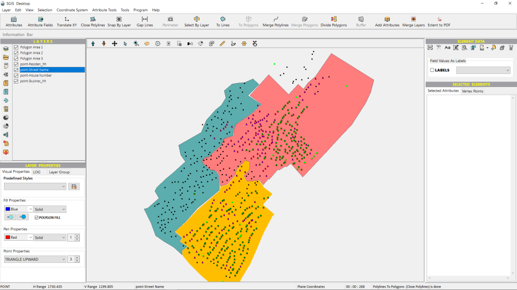
To illustrate the Point in Polygons criterion, we’ll use some example data. We have a telecommunications dataset that includes three distinct polygon areas, each connected to a telecommunication distribution cabinet. Within all three polygons, there are point features located across four different layers.
For our first example, we’ll focus on the Residen_hh Point layer. The user wants to filter all Residen points located inside Polygon Area 1, then those in Polygon Area 2, and finally, those in Polygon Area 3.
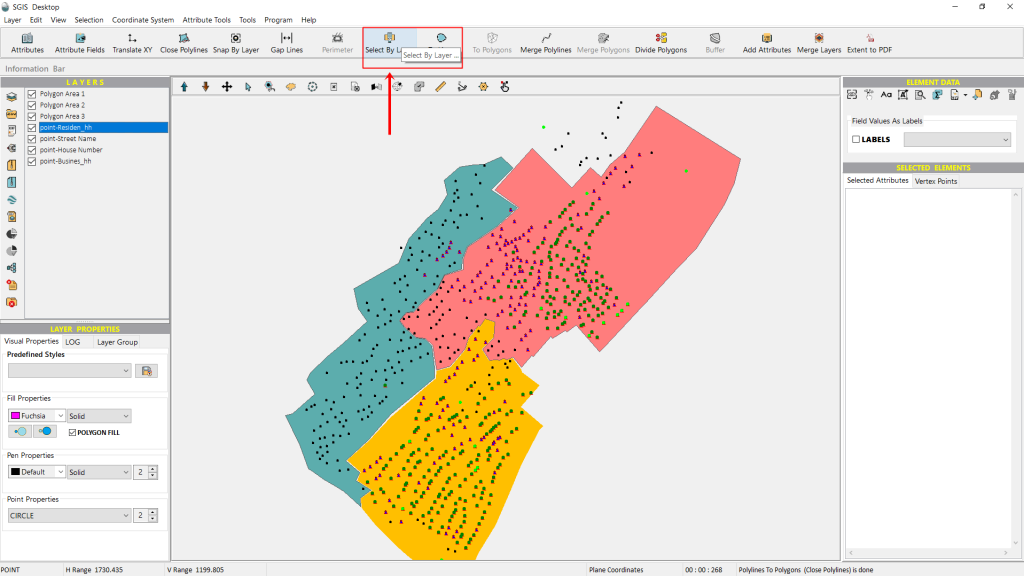
To do this quickly and effectively, we need to access the “Select By Layer” tool. You can find this tool in the Selection menu on the main toolbar, as well as in the toolbox located at the top of the user interface.
Let’s start by clicking on the function.
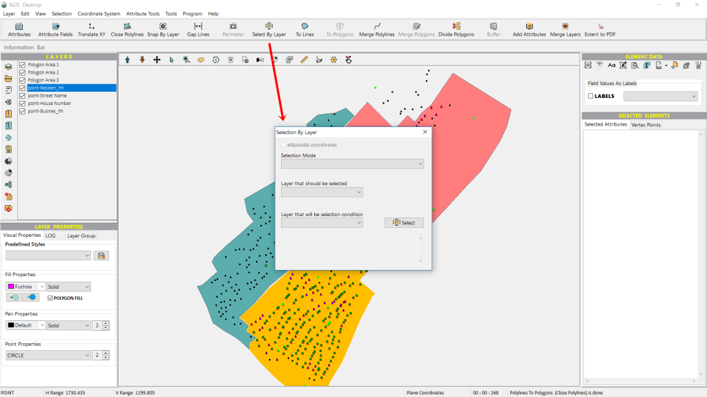
Once the function is activated, a dialog window will pop up. Here, users are prompted to choose the Selection Mode from a dropdown list, which includes all the spatial relationship criteria. We’ll select the criterion that’s appropriate for our example.
Next, users need to pick the ‘Layer that will be selected’.
This step sets up the spatial relationship criterion between two different layers, so it’s important to specify which layer’s features we want to select.
The third dropdown lets users choose the ‘Layer that will act as the condition,’ which defines the spatial relationship between the two layers.
Let’s start with the first selection.
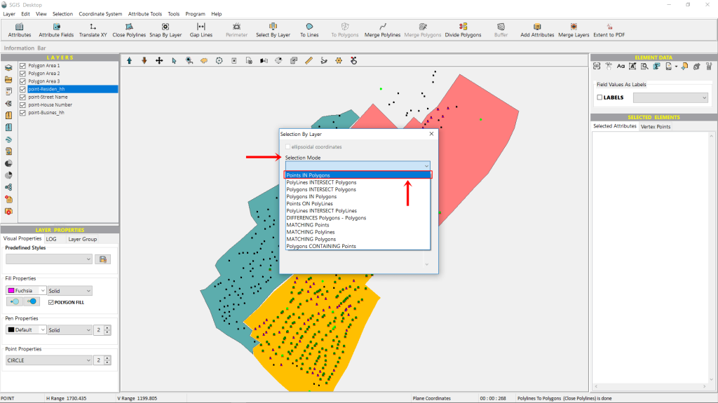
We’ll choose the first option from the dropdown list—Points in Polygons. This option lets us select point features that are found within one or more polygons. In other words, the Polygon layer can have multiple polygons.
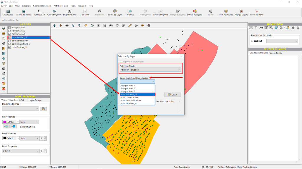
Next, we need to open the second dropdown list to choose the layer that contains the features we want to select and highlight. In our example, we want to select all Residen points located inside Area 1, so we’ll choose the ‘point-Residen’ layer.
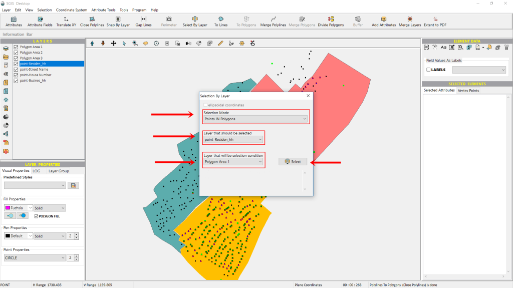
Naturally, the third dropdown option, the ‘Condition Layer’, will be the layer for ‘Polygon Area 1’. With these three settings configured, we just need to click on ‘Select’.
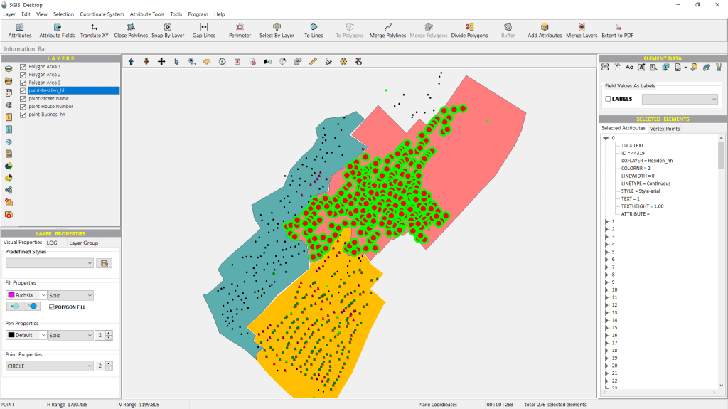
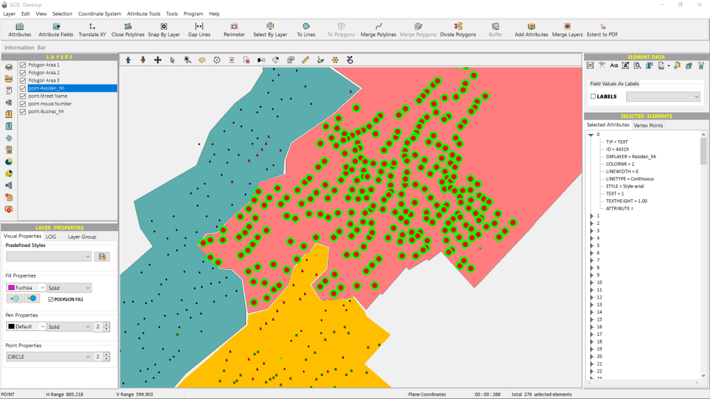
The points are highlighted in lime green, but this is a setting that users can customize to their liking.
The selected points can now be easily exported into a separate GIS layer for further processing. For instance, users can later open the attribute table and add new attribute fields to include relevant information.
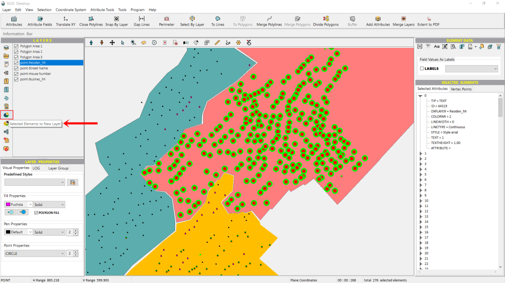
To do this, we’ll use the ‘Selected Elements in New Layer’ function.
This handy feature lets us create a new layer that includes the features we previously selected based on our chosen conditions. Let’s go ahead and click on it.
The function prompts us to enter a name for the new layer we’re creating. We’ll name it ‘Residen Points in Polygon 1’, as those are the points we were looking for.
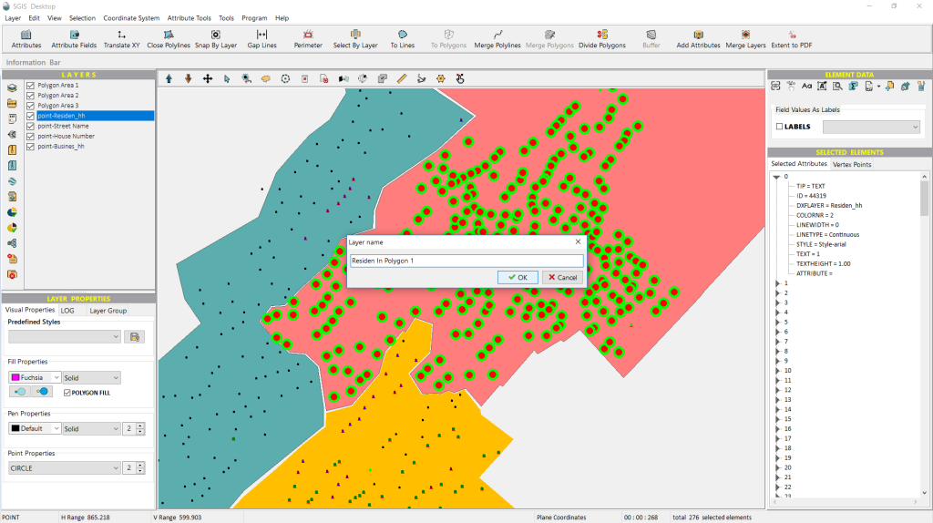
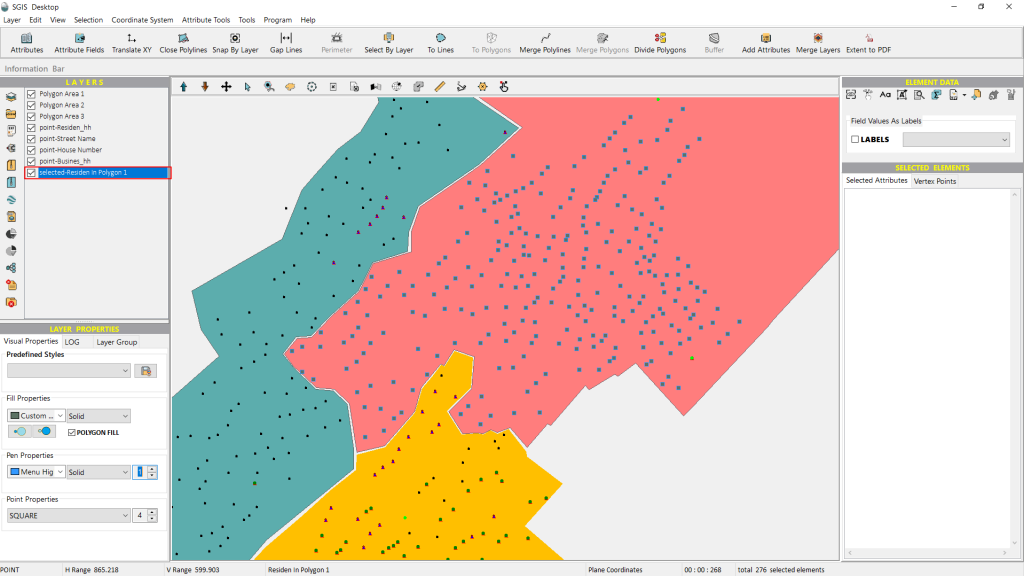
We click ‘OK,’ and with that, a new layer is created. The procedure is now complete.
Let’s demonstrate this spatial criterion with a practical example for utility and infrastructure projects. This tool allows us to analyze how different spatial features interact with each other.
In our example, we’ll show where heating network pipelines intersect with property boundaries; or pass through cadastral parcels. Each cadastral parcel is assigned its ownership, whether state-owned or private. It’s a quick and efficient way to highlight all the land parcels impacted by the network.
This is just one example, though. The same principle applies to roads (represented as polylines) intersecting land properties or buildings. Users can of course, analyze other infrastructure like power lines and pipelines, showing which properties they cross.
Now, let’s dive in and see how this is done in SGIS Desktop!
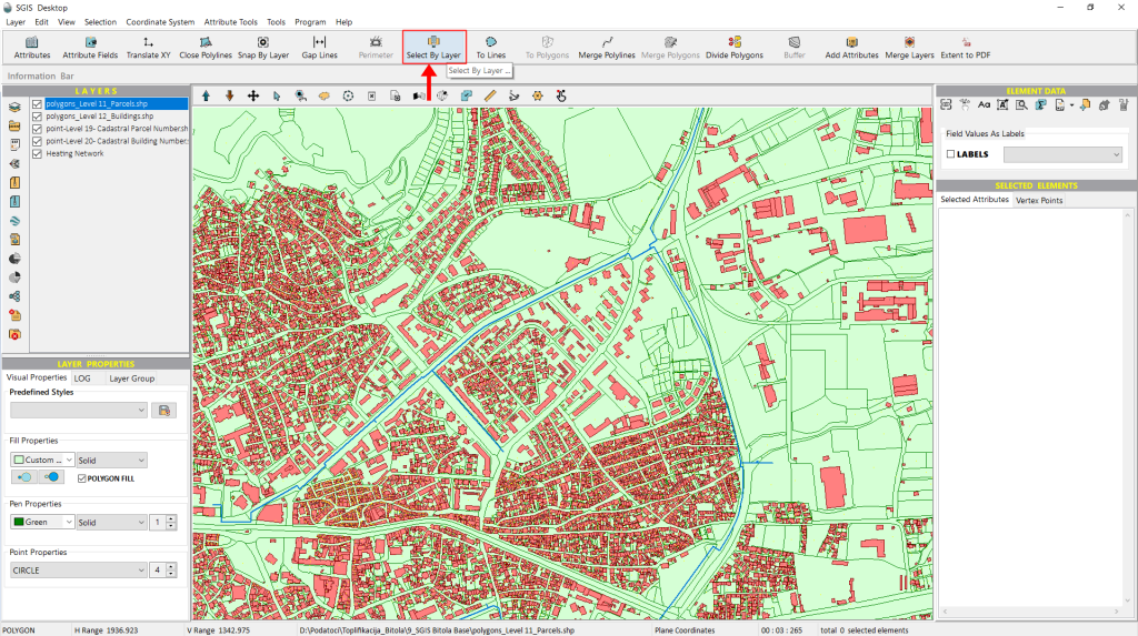
We’ve already loaded our dataset into SGIS, so we’re ready to jump right into the process. We have a SHP layer representing the heating network as polylines, along with a cadastral basemap that includes layers for land parcels and buildings. Our goal is to identify which parcels the pipeline network passes through.
To do this, we’ll use the ‘Select by Layer’ function. Let’s click on it and get started.
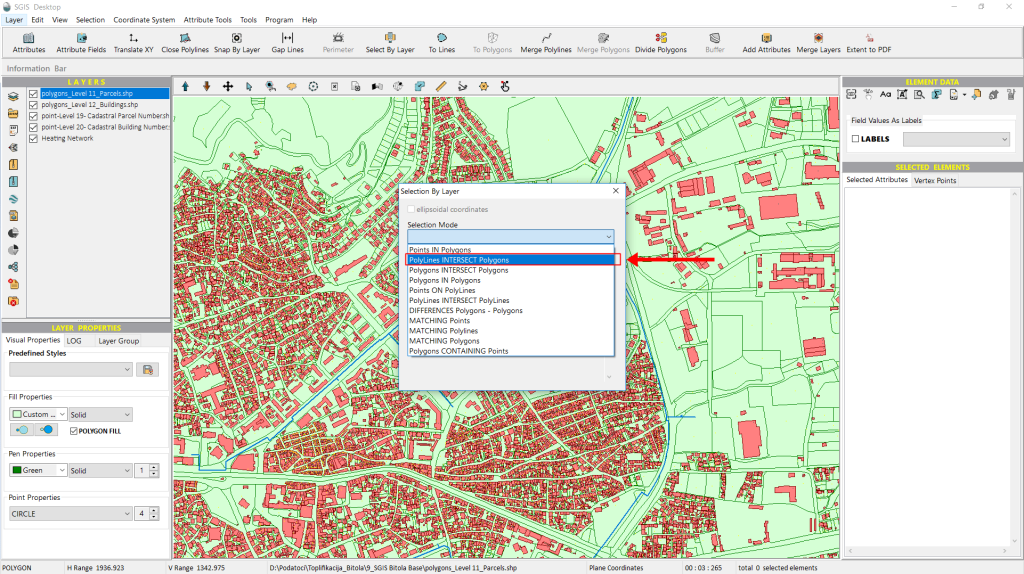
The Selection Dialog window will appear immediately. From the ‘Selection Mode’ dropdown menu, we’ll choose the second option, ‘Polylines Intersect Polygons.’ This option allows us to select all polygon features from one layer that are intersected by polyline features from another layer.
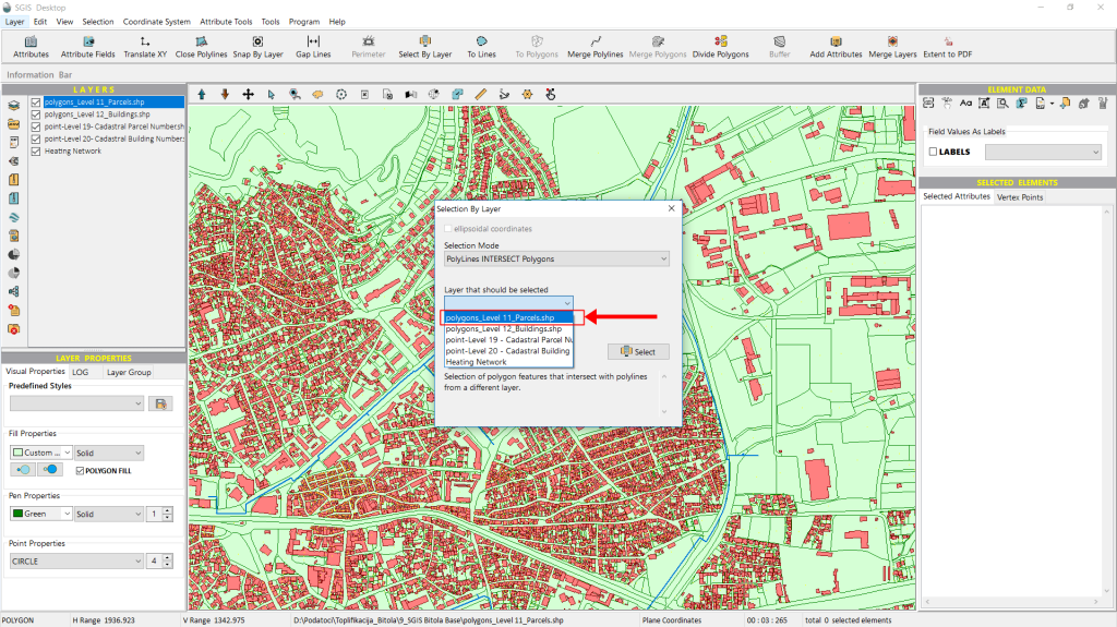
Once we’ve selected the ‘Selection Mode’, the next step is to choose the ‘Layer that should be selected’. Here, we specify which layer we want the features to be highlighted from. We’ll pick from a dropdown list that shows all the layers in the Layers panel. In this case, we’ll select the layer named ‘Level 11-Parcels’.
Next, we move on to the third option, the condition layer. This is where we specify the layer that will serve as the basis for applying the spatial relationship criterion. From the dropdown list, we’ll select ‘Heating Network’.
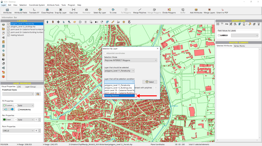
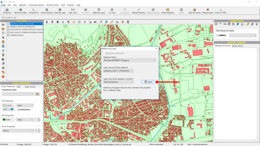
Once all three options are configured, we simply click on ‘Select’ to proceed.
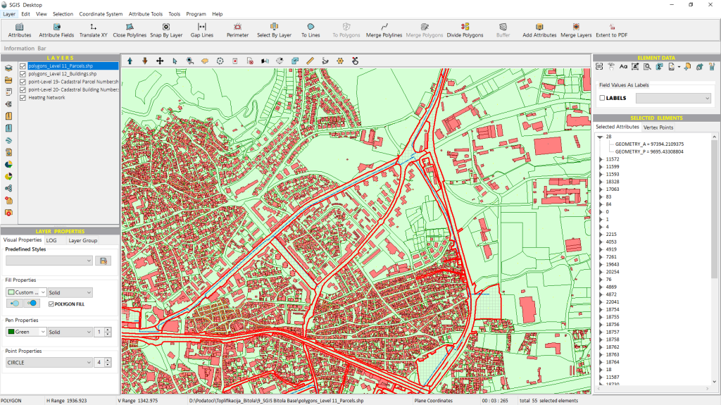
The features that meet the criteria are instantly selected and highlighted in the graphics panel. Additionally, these polygon features are listed in the ‘Selected Elements’ panel, allowing users to navigate through them individually and pan to each one as needed.
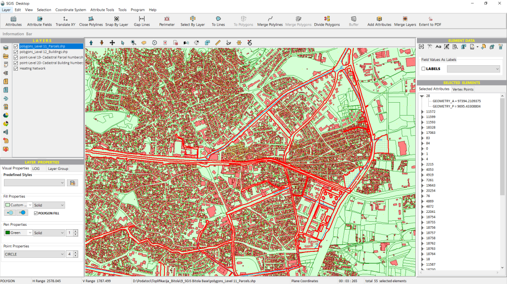
We have the option to separate these selected features into a new layer, which will be automatically created when we activate the ‘Selected Elements in New Layer’ function. This function is conveniently found in the ‘Layers’ Toolbox on the left side of the user interface. Let’s go ahead and click on it.
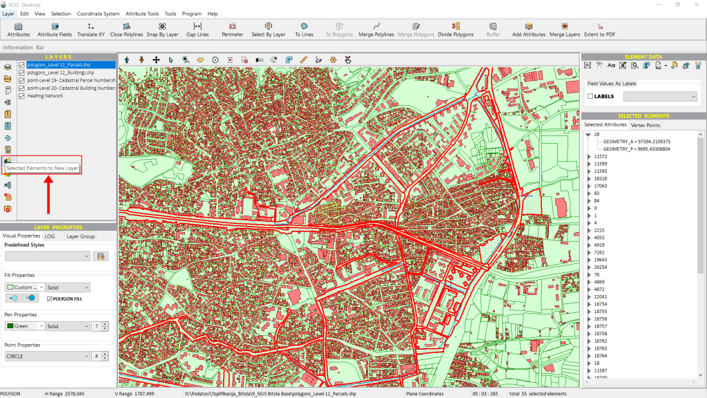
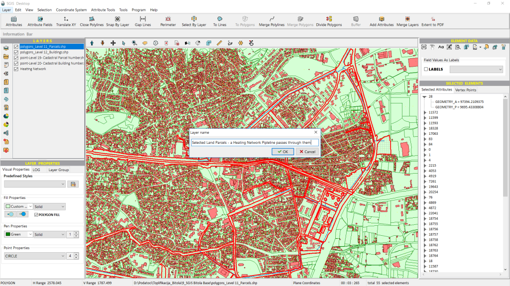
Once activated, the function will prompt us to enter a name for the new layer. After we do that, a new layer containing the selected features—in this case, the polygon features representing land parcels—will be created.
With that, the procedure is complete.
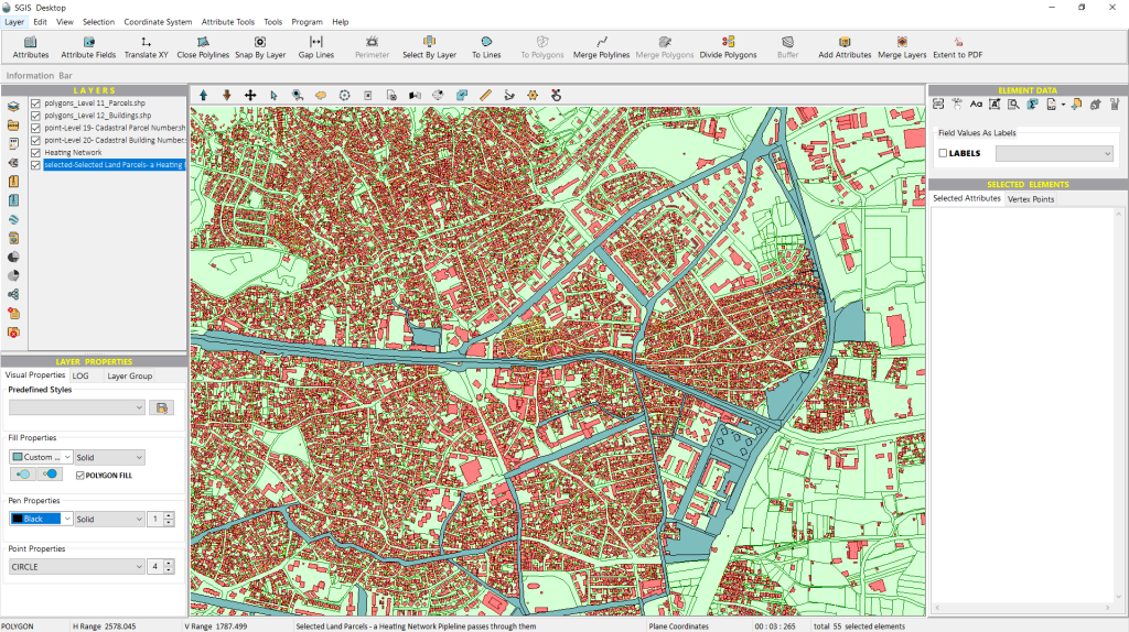
The “Polygons Intersect Polygons” spatial relationship criterion is a powerful tool for analyzing how different polygon features overlap within a specific area. For example, it can help identify where zoning areas (such as residential, commercial, or industrial zones) intersect with specific land use designations.
Similarly, it can show where protected areas, overlap with land designated for other uses, such as agriculture or development.
In cadastral mapping, this criterion allows users to see where property boundaries might intersect with municipal or administrative boundaries.
In our practical case, when planning large infrastructure projects like utility networks, this tool helps visualize how planned routes intersect with existing property boundaries, aiding in optimization and minimizing disruption.
Now, let’s dive into how this is done;
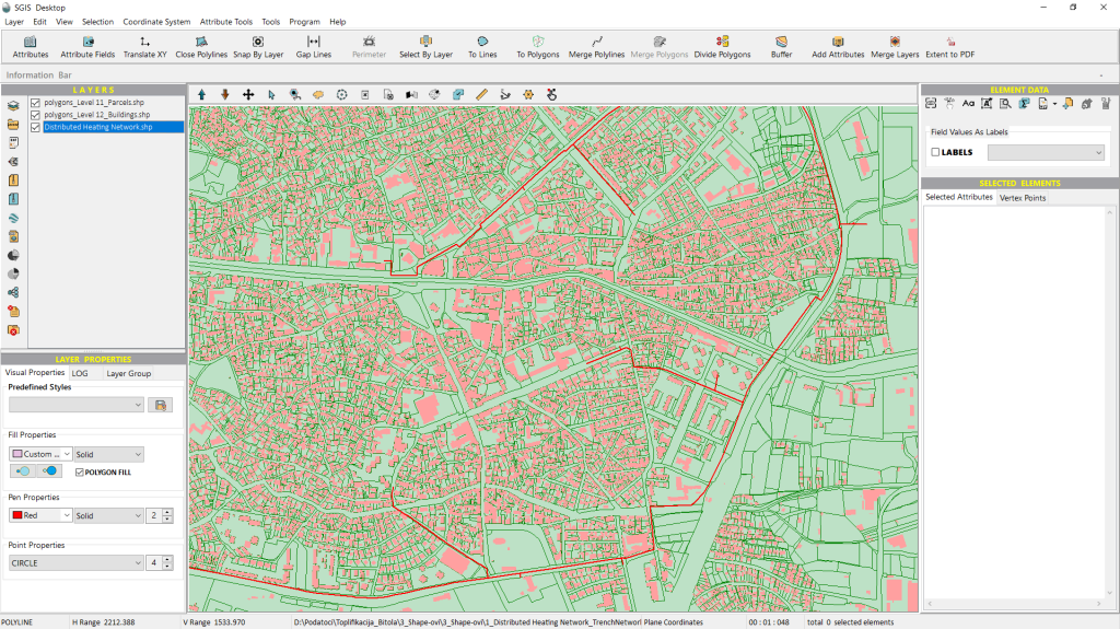
Since we already have our dataset loaded from the previous example, in this case, we need to create a buffer around the heating network pipeline to identify which land parcels fall within the designated project area. We’ll set the buffer to 10 meters on both sides of the pipeline and check which land parcels are impacted by the project.
To begin, we’ll open the ‘Buffer’ function.
This function is easily accessible in the main toolbar at the top of SGIS Desktop’s user interface.
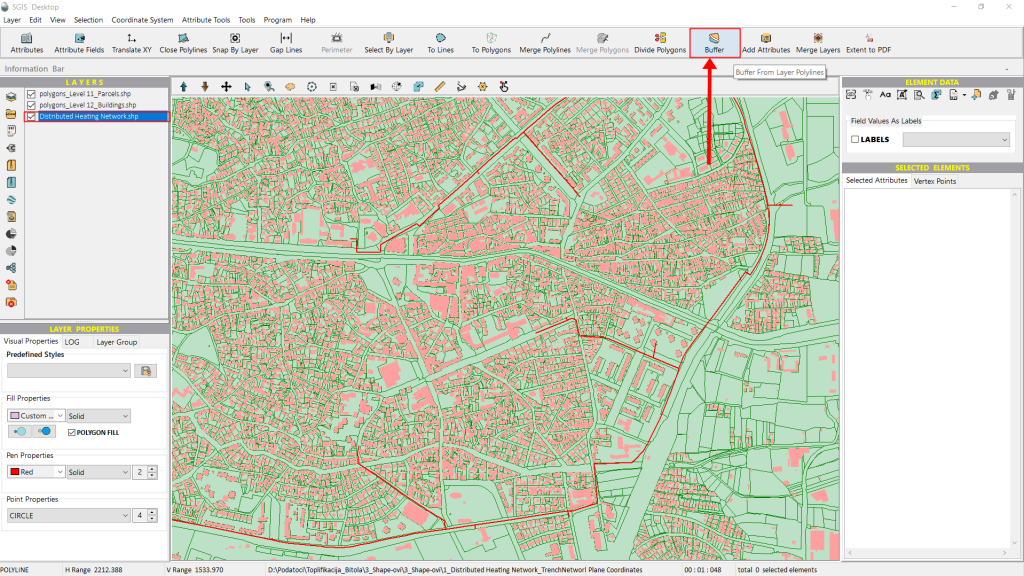
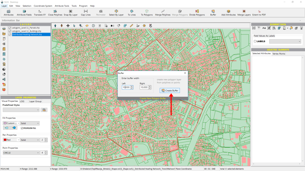
After configuring the settings, we click ‘Create Buffer’.
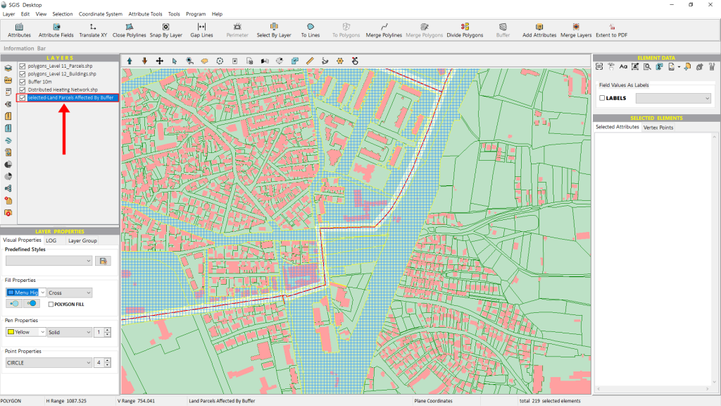
A new layer with the buffer polygon immediately appears in the Layers List. Now that the buffer is created, we can use the ‘Select by Layer’ function to identify where the two polygon layers overlap and intersect.
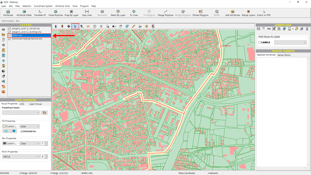
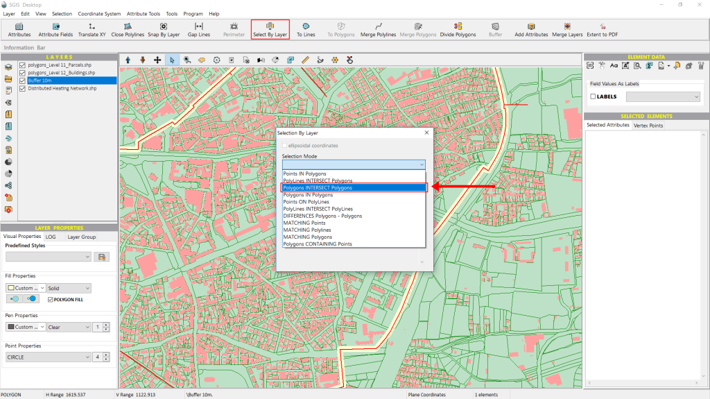
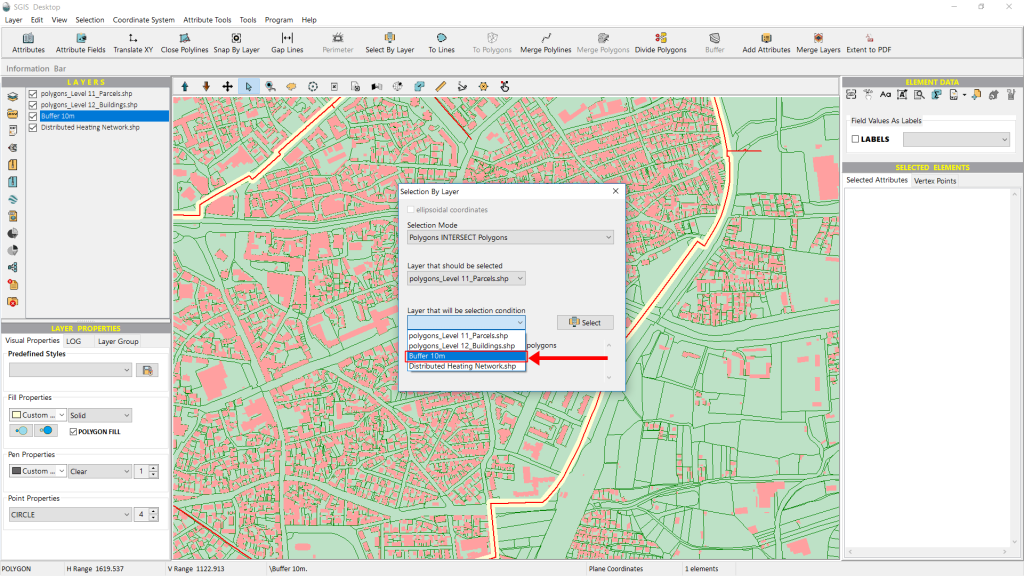
When the ‘Select by Layer’ dialog window opens, we start by choosing our mode from the ‘Selection Mode’ dropdown menu, selecting ‘Polygons Intersect Polygons’.
Next, under the ‘Layer to be selected’ dropdown, we choose ‘Level 11 – Land Parcels’.
For the third dropdown, we select the ‘Buffer 10m’ layer.
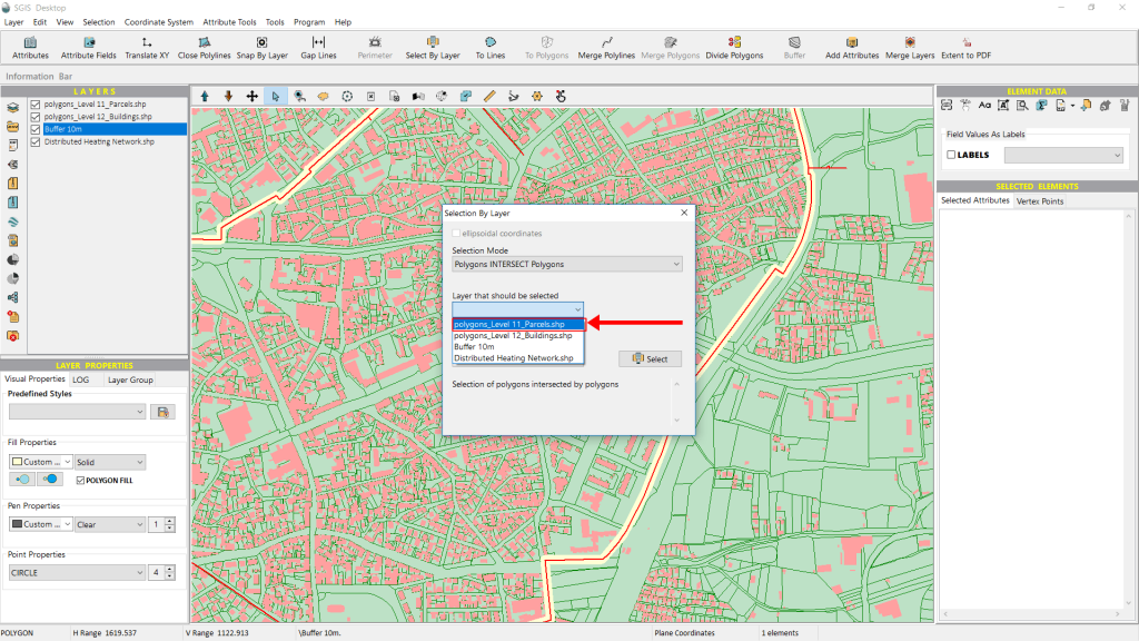
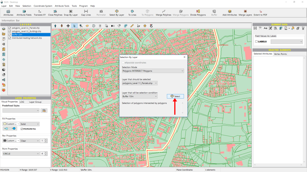
Finally, we click ‘Select’ to finish the process.
All polygon features that meet the criteria will instantly be selected and highlighted in the Graphics panel.
In this example, the highlighted polygons appear in red, though this is fully customizable and can be adjusted based on user preferences.
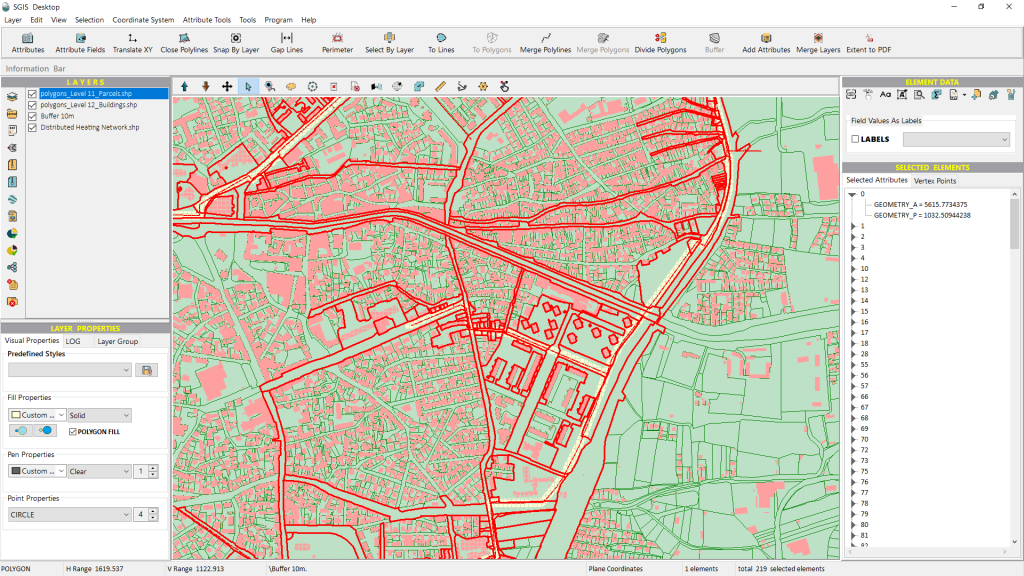
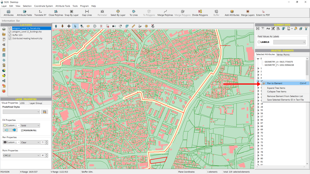
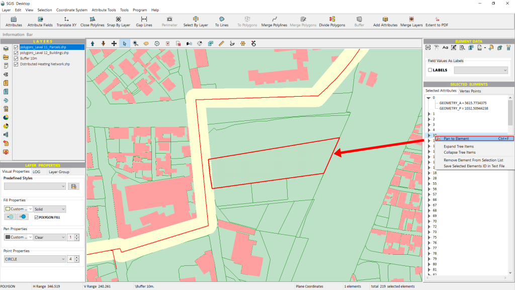
One great feature of SGIS is the ‘Pan to Element’ function found in the Selected Elements panel. After making a selection, the highlighted elements will not only be visible on the graphics panel, but they will also be listed in the Selected Elements panel. Users can click on each element individually, and its attributes will be displayed in a convenient tree-like format.
This is particularly useful when you want to quickly check the attribute values of a selected element without having to open the entire attributes table.
If you right-click on any item in the list, a menu will pop up, and the first option will be ‘Pan to Element.’ This feature makes it easy to zoom in on the selected element in the graphics panel, eliminating the need for a manual search.
We can easily separate all the polygons into a new layer using the one-click function ‘Selected Elements in New Layer’ for further processing and analysis of their geometry and attributes. After naming the new layer, it will be created instantly, and with that, we’ll wrap up this procedure.
The “Polygons In Polygons” spatial relationship criterion is useful for analyzing how certain polygon features are fully contained within others. For instance, it can determine which parcels of land fall entirely within specific zoning areas or help identify properties located completely within protected regions, like nature reserves or conservation zones.
In cadastral analysis, it can highlight smaller land parcels (such as subdivided lots) that fall entirely within larger municipal or administrative boundaries.
In our case, we have a cadastral dataset that includes both land parcels and building polygons. The building polygons represent all the buildings in the village, while the land parcels are only for a portion of the area, designated for specific use.
Our goal is to compare the two layers to see which buildings fall inside the designated land parcels and which ones, are located outside.
Let’s get started;
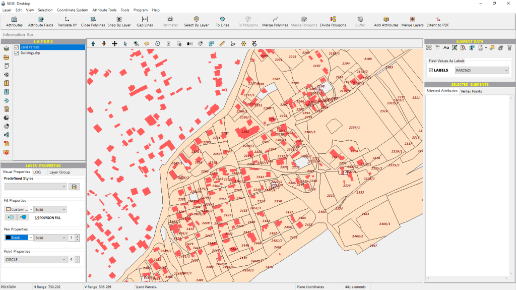
The land parcels layer, consisting of multiple polygon features, has been successfully loaded, along with the buildings layer.
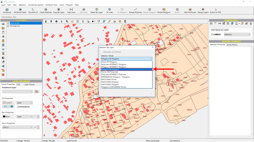
Now, we’ll open the ‘Select by Layer’ function. First, we click on the ‘Selection Mode’ dropdown to reveal the options, and we select “Polygons In Polygons”.
Next, from the second dropdown list, we choose ‘Buildings’ as this is the layer we want to select features from.
Lastly, for the condition layer, we’ll select the ‘Land Parcels’ layer. Since there are only two layers in the Layers panel, this choice is straightforward.
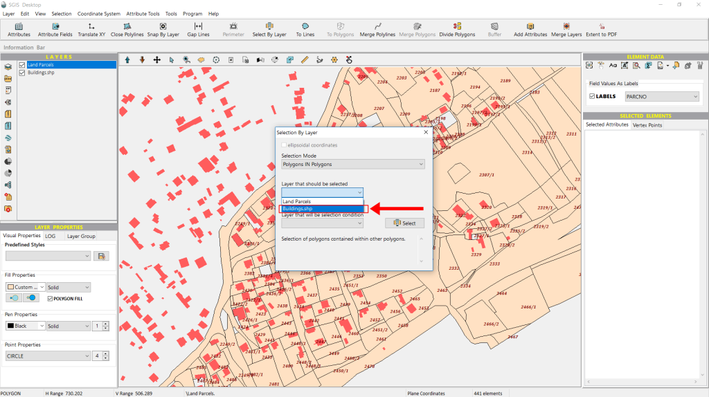
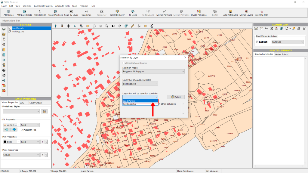
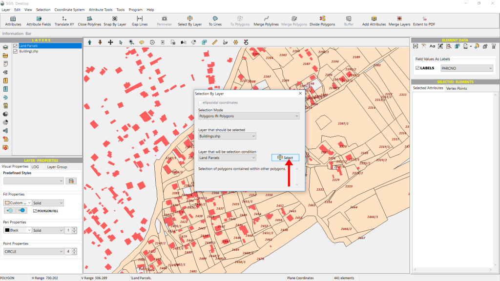
Next, we click on ‘Select’ to continue with the process.
As shown in Fig.39, all building polygons that meet the criteria are immediately selected and highlighted.
Additionally, the selected elements are displayed in a tree-like list in the ‘Selected Elements’ panel.
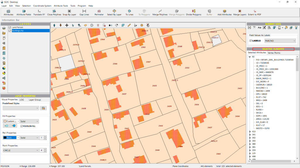
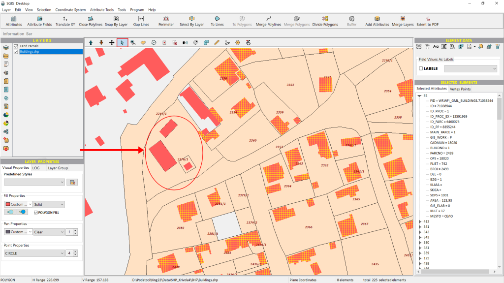
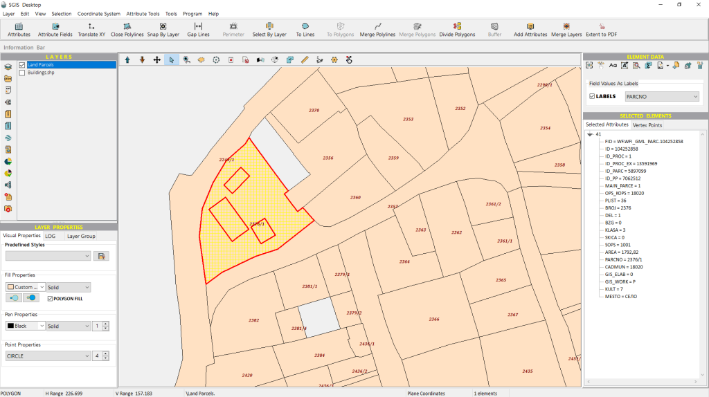
An interesting detail in this case is that, as we zoom out, a few buildings remain unselected. This isn’t an error. If we temporarily disable the Buildings layer from the Layers panel, we can see that these buildings don’t meet the criteria because the areas they overlap aren’t polygons, but gaps within a larger polygon.
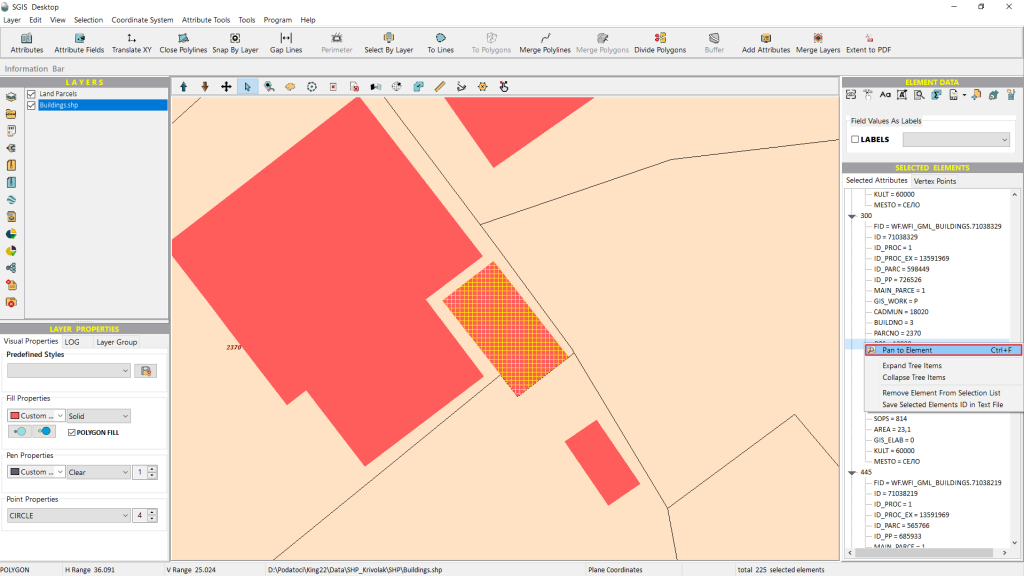
We can select an element from the Selected Elements list, right-click on it, and choose ‘Pan to Element’. This will take us directly to that specific element, highlighting its geometry and location.
There are additional options, such as expanding or collapsing the tree items, removing an element from the selection, or exporting the element’s ID as a text file.
For demonstration purposes, we’ll now move ahead and use the ‘Unselected Elements in New Layer’ function. This will create a new layer in the Layers panel, containing all elements that were not part of the previous selection process.
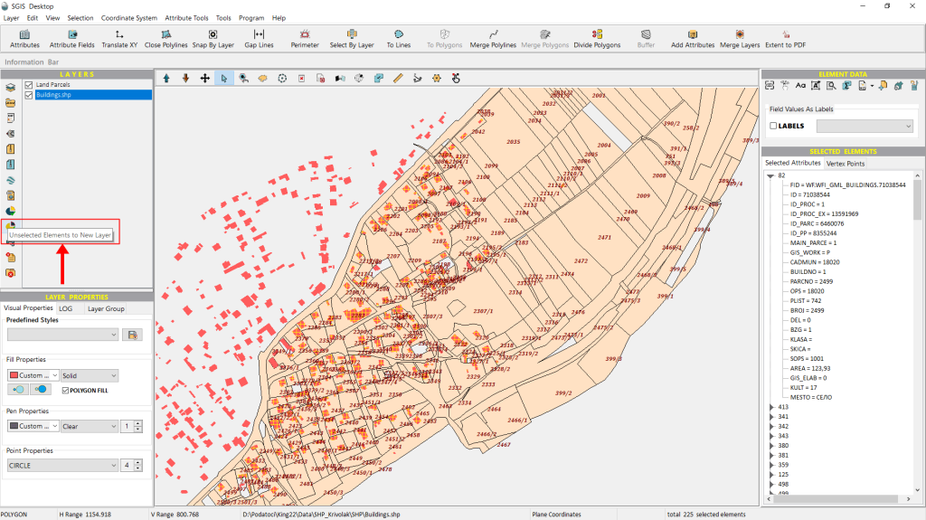
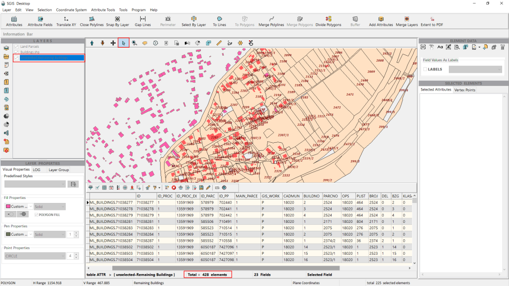
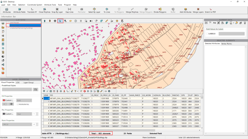
As shown, the new layer is created instantly. Upon opening the attribute table, we can see that this layer contains 428 elements, or building polygons. The Info bar in the bottom-right corner shows the number of selected elements from our process—225 building polygons.
If we compare this to the original buildings layer, which contains 653 building polygons, the numbers align perfectly. We selected 225 polygons that overlap with land parcels, while 428 polygons did not meet that criterion.
With this, we successfully complete the procedure.
This criterion is particularly useful for analyzing the spatial relationship between point features and polylines, helping to determine whether specific points are directly on or along a polyline feature.
In this practical example, we’ll work with point data gathered through field measurements for the maintenance of a telecommunications network, specifically focusing on underground optical cable pipelines. The scenario involves an optical cable network, where each shapefile represents a different cable segment.The point coordinates represent the actual field data collected for maintenance purposes.
Our task is to overlay these points onto the network and identify which points align with specific cable segments. Let’s explore how this process is carried out using SGIS Desktop.
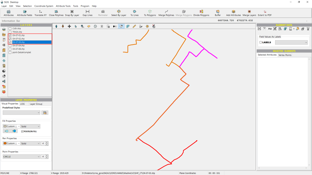
All the shapefile layers have been imported into the software, but they are initially disabled. To provide a clearer view of the cable segments, we’ll enable them one by one. In Fig.46, two cable segments are now visible in the Graphics panel.
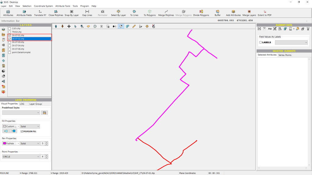
Next, we’ll continue enabling each layer one by one until all five cable segments are visible. Each segment is color-coded differently for easy distinction.
Finally, we’ll enable the point layer containing the field measurement data.
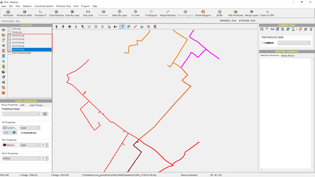
The point data consists of measurements taken along the trench of the telecommunications network, with additional points for segments that aren’t currently displayed. All of this data is stored in a single CSV file, rather than being divided by segments.
As shown in Fig.49, there are a large number of points to work with, so we need the quickest and most efficient way to sort these points by their respective segments.
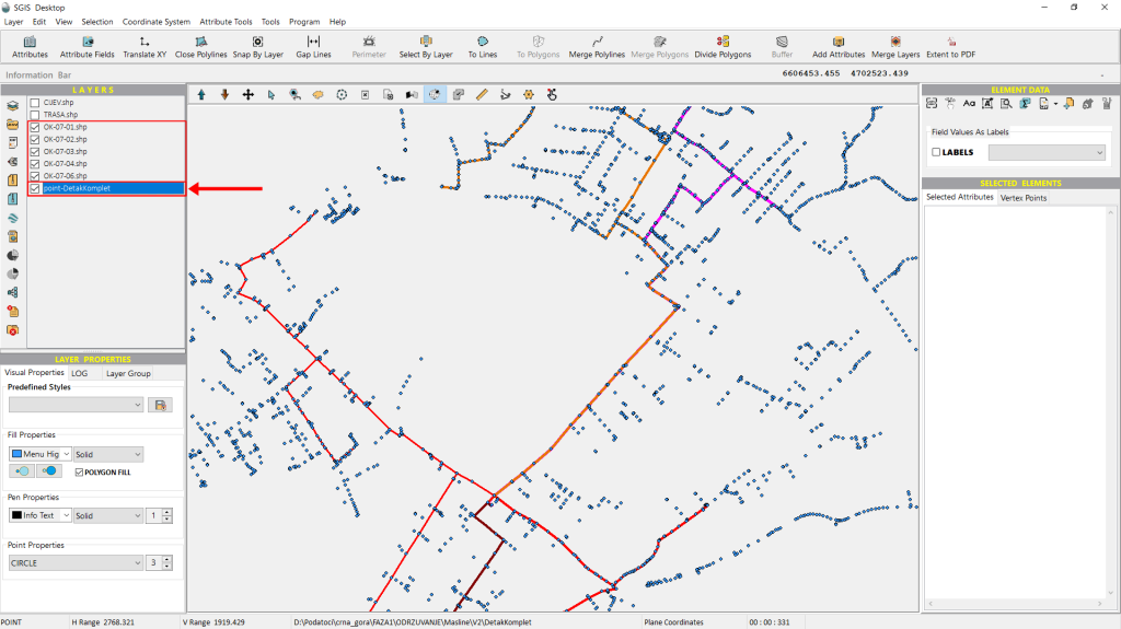
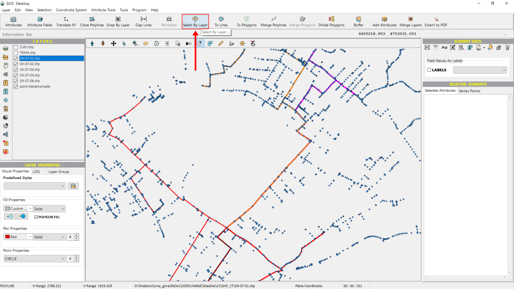
The ‘Select by Layer’ tool, specifically the ‘Points On Polylines’ option, offers a quick solution that saves us the hassle of manually drawing polygons around each cable segment to isolate points. Instead, we can easily set our selection mode and criteria—for instance, finding the points that fall directly on Segment 1.
So, let’s start with the first segment: We begin by opening the ‘Select by Layer’ function.
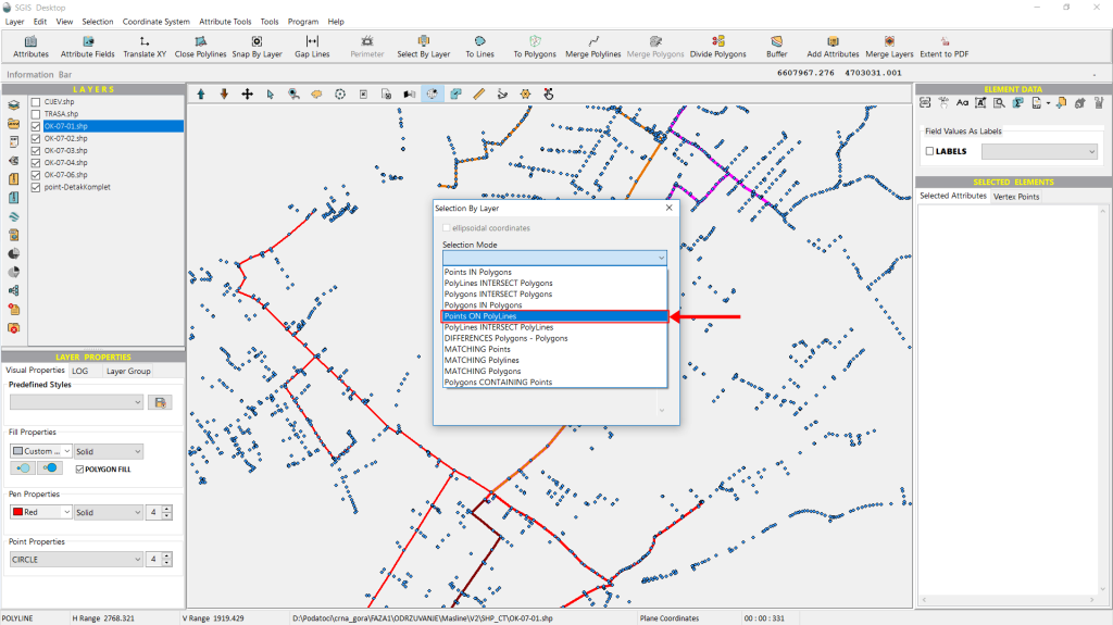
Next, we select the “Points On Polylines” option from the dropdown list and click on it to proceed.
Next, we move to the second dropdown menu and select the Point layer, since that’s where we want to choose the points for our analysis.
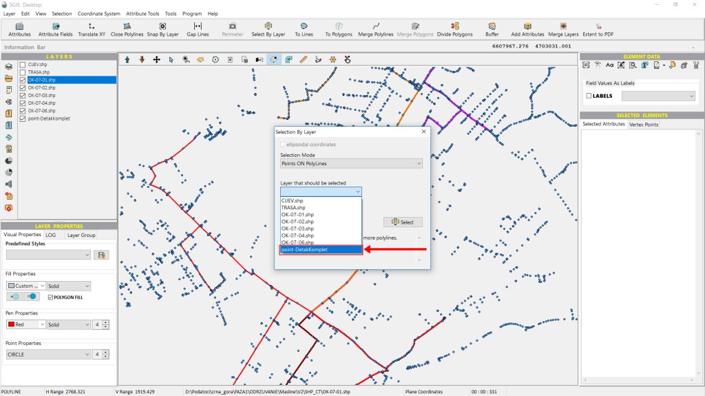
Finally, we select the cable segment shapefile layer from the third dropdown menu, which will serve as the condition layer for our selection. With five segment layers loaded in the Layers panel, we’ll begin by choosing the first one.
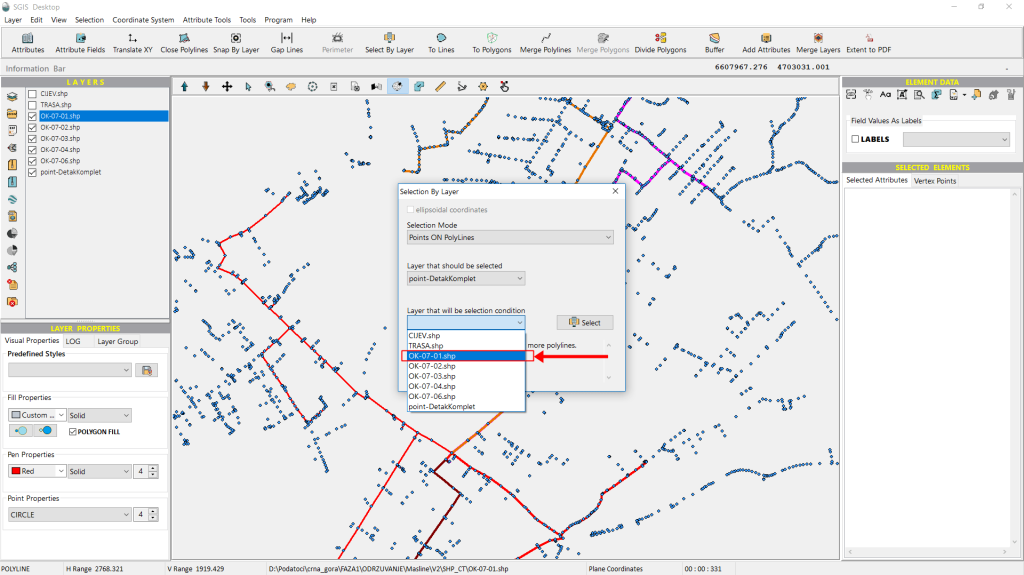
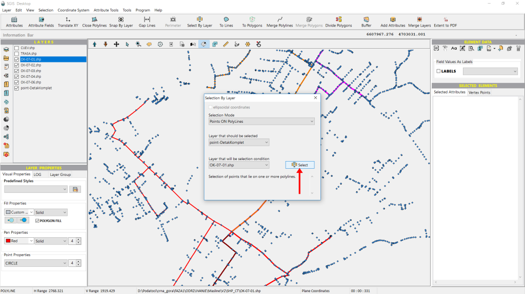
We then click on ‘Select’.
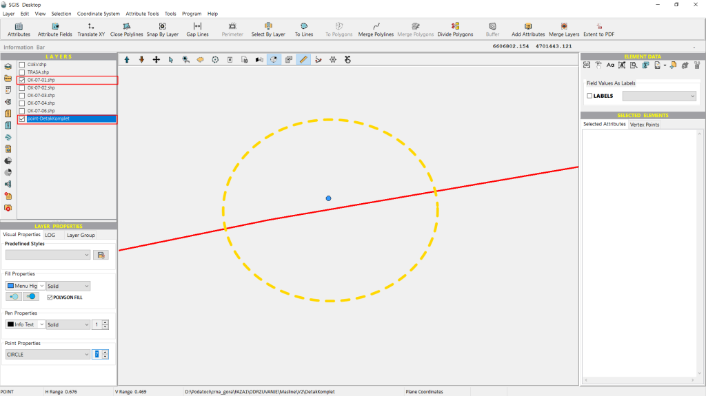
However, despite the point elements appearing to lie on the polyline segments, none of the points are selected.
This is because they aren’t precisely positioned on the polyline. By zooming in closely, we can see that the point features are not exactly aligned with the polyline.
In Fig. 55 and Fig.56, the misalignment is clearly visible, as only the two layers involved in the selection process remain enabled, making it easier to see that the points do not align with the polyline.
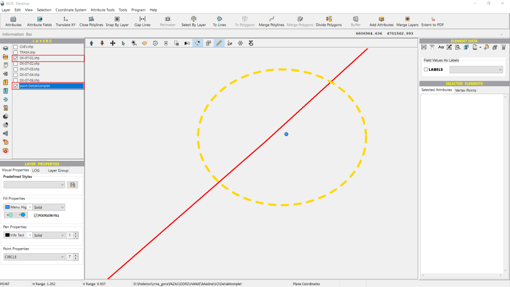
In situations like this, we would typically use the ‘Snap by Layer’ function, which allows us to resnap the polyline vertices to the points based on a defined proximity. However, for demonstration purposes, we’ll go ahead and repeat the selection process with the third segment layer from the Layers list.
Once again, we open the ‘Select by Layer’ dialog and set the same options as before. The only difference this time is that we’ll choose the third segment from the list for the third option.
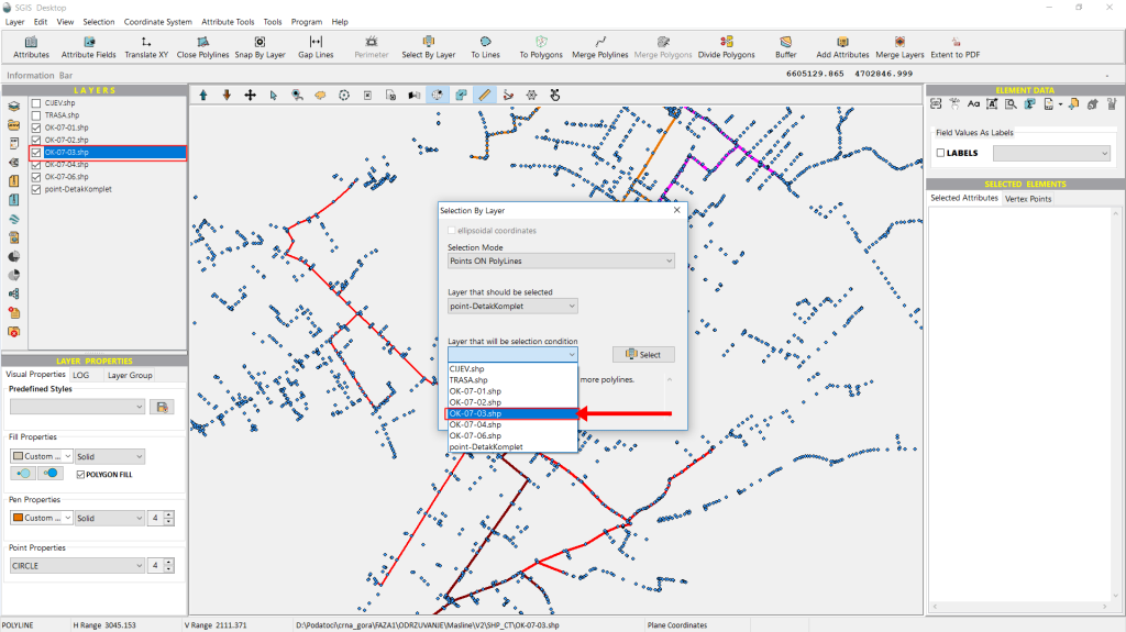
We click on ‘Select,’ and right away, the points are selected and highlighted on the Graphics panel. Additionally, all selected points appear in the ‘Selected Elements’ panel.
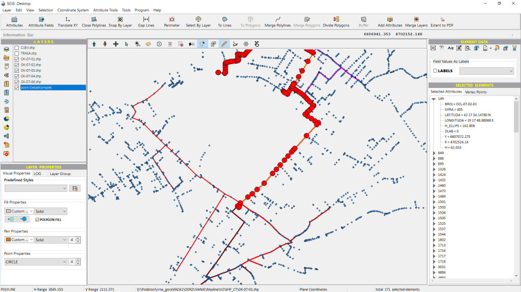
We can either review each point one by one or export all of them into a separate layer for further processing.
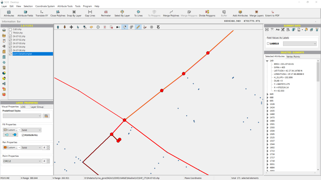
We decide to export all the selected points into a new separate layer using the ‘Selected Elements in New Layer’ function.
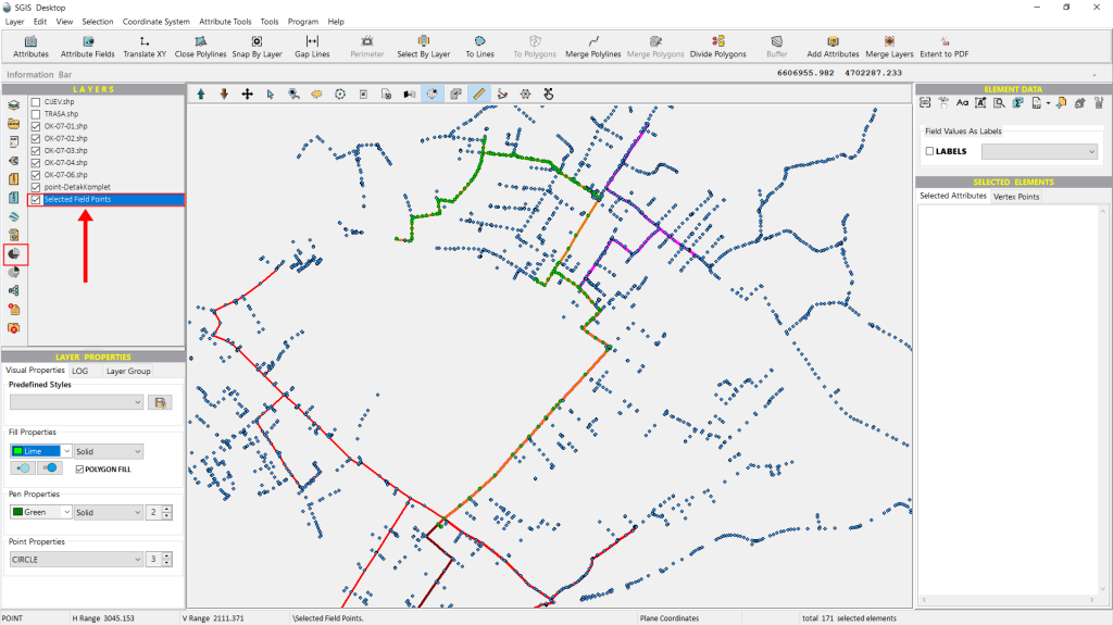
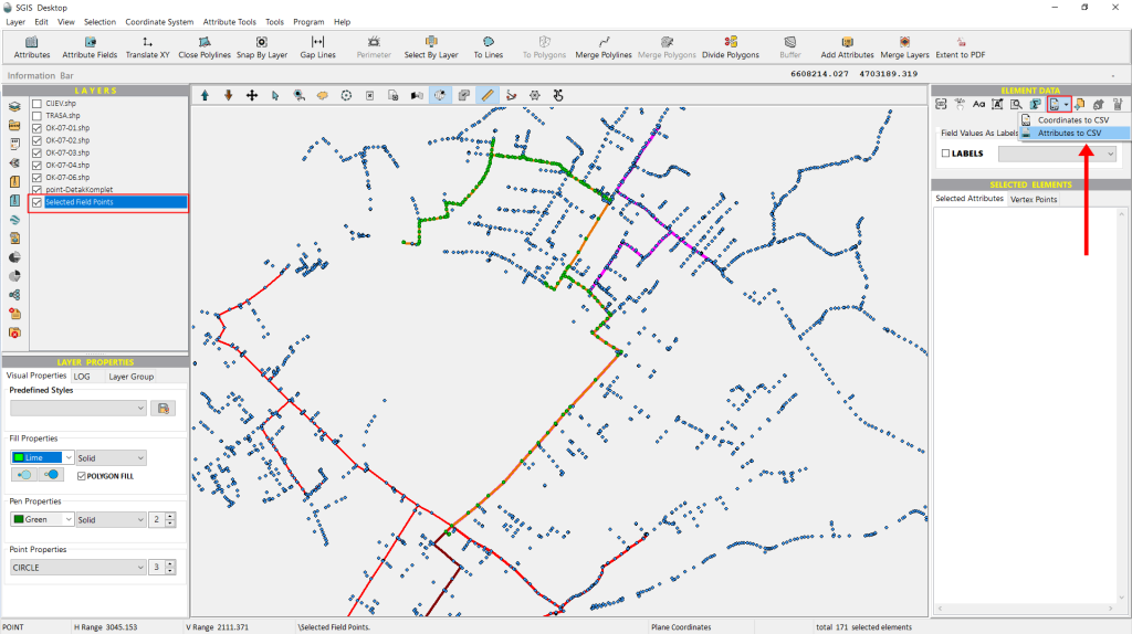
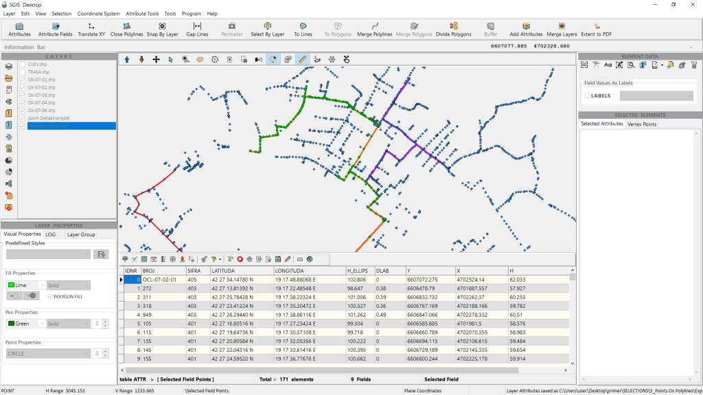
Once the new layer is created with only the filtered and selected points based on specific criteria, we can easily export the layer’s coordinates and attributes as separate CSV files. To do this, simply click on the ‘Coordinates to CSV’ or ‘Attributes to CSV’ option found in the ‘Element Data’ toolbox.
With this, we’ve successfully completed the procedure.
‘Polylines Intersect Polylines’ refers to a spatial relationship criterion where two or more polyline features intersect or cross each other at one or more points in a GIS environment. This criterion is used to identify places where different linear features, such as roads, pipelines, or utility lines, physically cross or share common points.
In GIS analysis, this helps ensure that certain connectivity, overlap, or crossing relationships are correctly represented between layers, aiding in tasks like network analysis, infrastructure management, and spatial data validation.
Our practical example involves working with a Detailed Urban Plan in a digital CAD format. This plan consists of multiple layers, including building lines, land parcels, existing streets, buildings, stormwater drainage, water supply systems, and more. Among these layers are underground power cables and underground telecommunication lines—both optical and copper. The telecommunication lines are categorized as either existing or planned.
In this example, we’ll focus on determining if, and where, the planned telecommunication optical cable trench intersects with the existing underground electrical power cables. These power cables are buried for electricity transmission and distribution, making this analysis crucial. It’s a high-risk task, as digging and trenching without proper knowledge of existing cables can be hazardous for field workers.
Our second analysis will focus on identifying which land parcels the existing new optical cable crosses. This is important for future assessments related to land ownership and legal rights.
Let’s dive in. SGIS integrates these capabilities into both SGIS Desktop and SGIS v.R software.
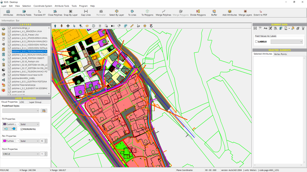
Let’s begin by accessing the ‘Select by Layer’ function. You can find it on the main toolbar of the user interface—just click to open it.
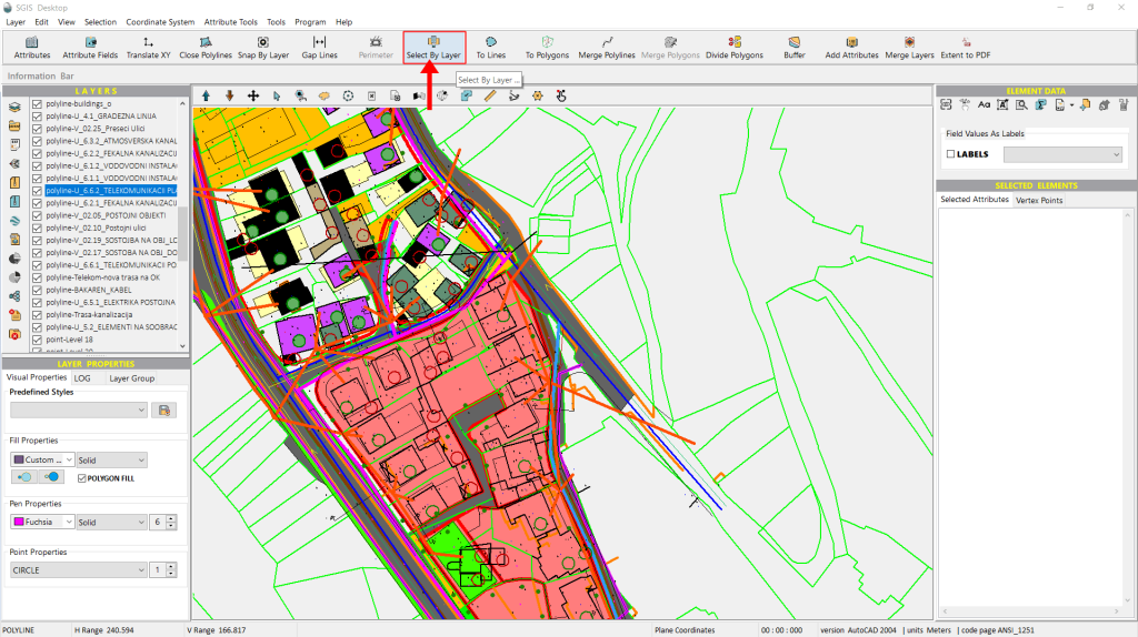
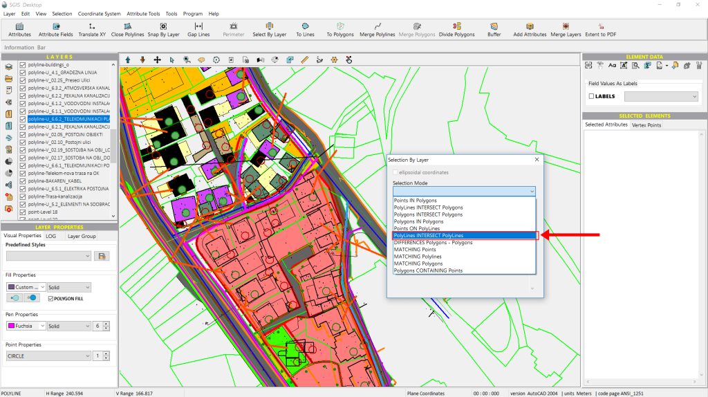
After activating the function, a dialog window will appear. From there, we simply open the dropdown list and choose the ‘Polygons Intersect Polygons’ spatial relationship criterion.
From the second dropdown list, we’ll choose the planned telecommunications optical cable trench layer, as that’s the focus of our spatial selection.
Then, from the third dropdown list, we’ll select the layer representing the underground electrical cables. Finally, we click ‘Select’ to execute the selection.
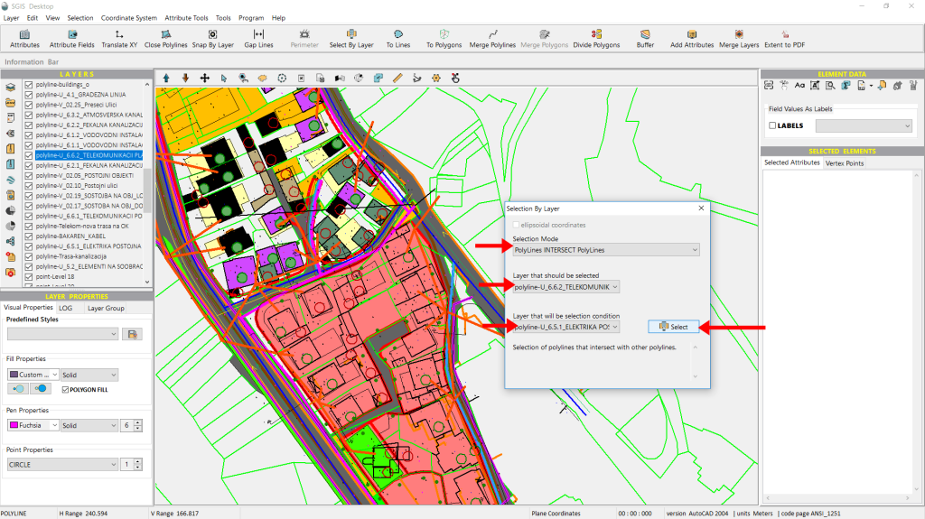
As we can see, two optical cable trenches are highlighted on the graphics panel. The default highlight color is red, but as mentioned before, this can be customized. In this example, with so many layers, the selected lines may not stand out clearly.
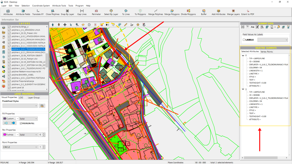
However, they are listed in the ‘Selected Elements’ panel on the right side of the interface.
To make it easier to work with the layers, we’ll export the selection as a separate layer using the ‘Selected Elements in New Layer’ function. This will allow us to disable all other layers, making the selected elements much clearer in the graphic panel.
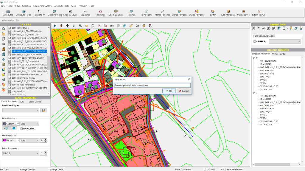
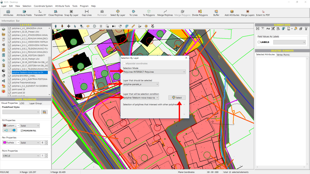
Once we’ve completed the previous step, we can head back to the ‘Select by Layer’ function to repeat the process with different layers. This time, we want to identify and isolate the land parcels that the existing telecommunications cable trench crosses. These parcels are crucial for further analysis regarding land ownership and legal rights.
We’ll use the same selection mode—‘Polylines intersect Polylines’—since this is a CAD file, and the land parcels are represented as polylines rather than polygons. For the ‘Layer to be selected’, we’ll choose ‘Land Parcels’, and the condition layer will be the existing telecommunications cable trench. Now, we simply click on ‘Select’.
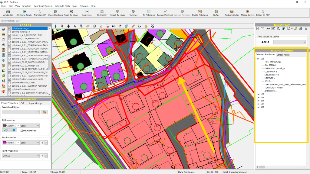
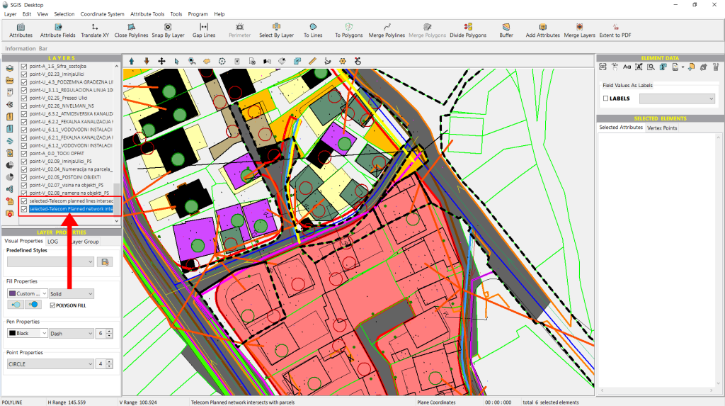
The land parcels that meet our criteria are quickly selected and highlighted on the graphics panel. They’re also listed in the Selected Elements tree for easier management. Next, we’ll separate them into their own layer for better organization.
Next, we’ll disable all the layers in the Layers panel and only open the ones necessary for our analysis. This includes the land parcels, the planned and existing telecommunications cable trench, the underground electric power cable layer, and a layer for additional elements like pavements and similar polylines. We will also include the two separate layers created from our previous selections: the layer where the planned trench intersects with the electric cable and the parcels that the new telecommunications cable passes through.
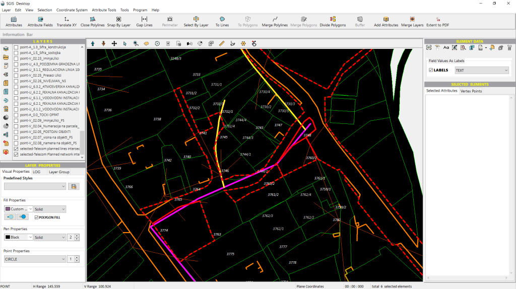
By narrowing down the layers, our workflow becomes clearer for further processing. As shown in Fig.72, the interface resembles a CAD environment, even though it operates within a GIS framework, allowing users to input attributes into each layer.
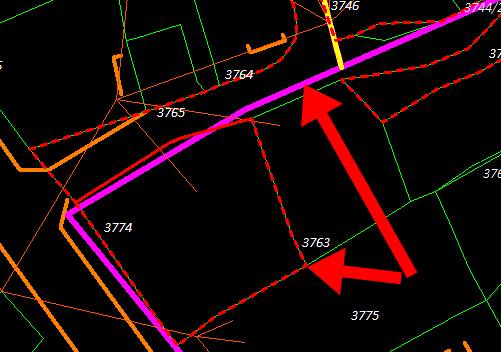
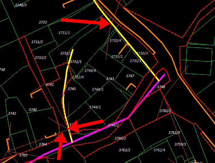
We’ve included Fig.73 and Fig.74 to enhance visual clarity.
In Fig.73, the existing telecommunications trenchline is prominently displayed in a fuchsia color, with the separated land parcel polylines overlaid in a dashed red.
Fig.74 showcases the planned telecommunications cable trench in a bold yellow line, while the electrical cable network is represented by a thin sepia-colored polyline.
With this, we have completed the procedure.
‘Differences – Polygons with Polygons’ refers to a spatial relationship in GIS that calculates the difference between two polygon layers. This relationship identifies areas in one polygon layer that do not overlap with another polygon layer.
For example:
- If you have two polygon layers, the “difference” operation subtracts the areas where the polygons overlap, leaving only the parts unique to one of the layers.
This method is commonly used in GIS to identify excluded areas or highlight distinctions between regions. It has applications in urban planning, environmental monitoring, and land use analysis.
Here’s how it works:
When you apply the difference operation, the area of one polygon is subtracted from another. The result is a new polygon representing the part of the first polygon that does not overlap with the second.
A random example:
- Input:
- Polygon A: A city park.
- Polygon B: A new construction site that overlaps part of the park.
- Difference Result (A – B):
- The output will be the part of the park (Polygon A) that isn’t covered by the construction site (Polygon B).
In our example, we’re working with two building layers. The first layer includes building footprints extracted from CAD sources and satellite imagery, while the second layer contains the official building footprints registered in the Government’s Real Estate Cadastre. Together, these layers represent the complete building layout for an urban municipality area.
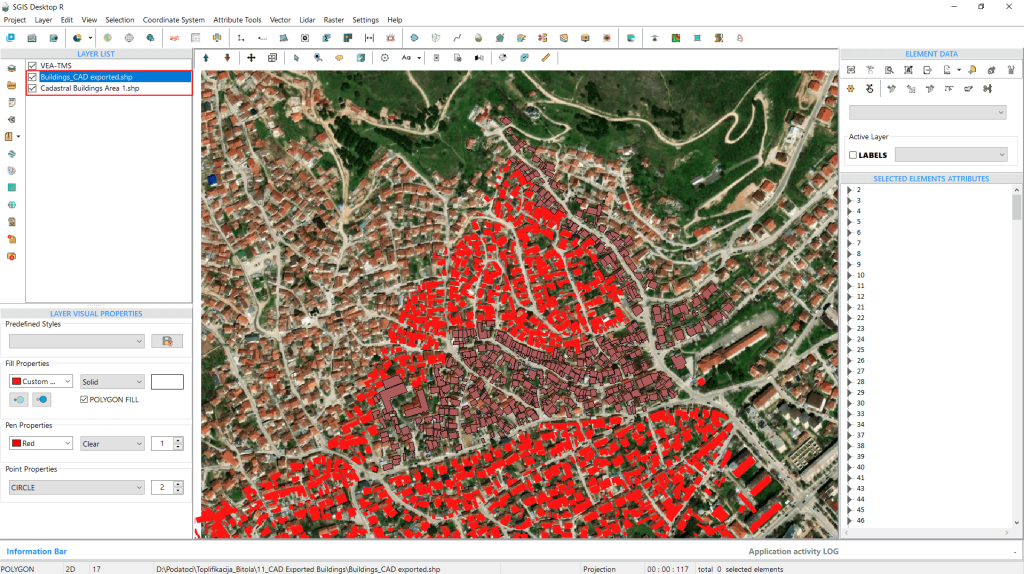
To demonstrate SGIS’s spatial relationship criteria, we’ll use the ‘Select by Layer’ option called Differences – Polygons with Polygons. Our goal is to select all the building polygons from the first layer that don’t overlap with those in the second layer.
In the previous examples, we used SGIS Desktop. Now, we’ll switch to SGIS v.R to show that these functions are available in both versions of the software.
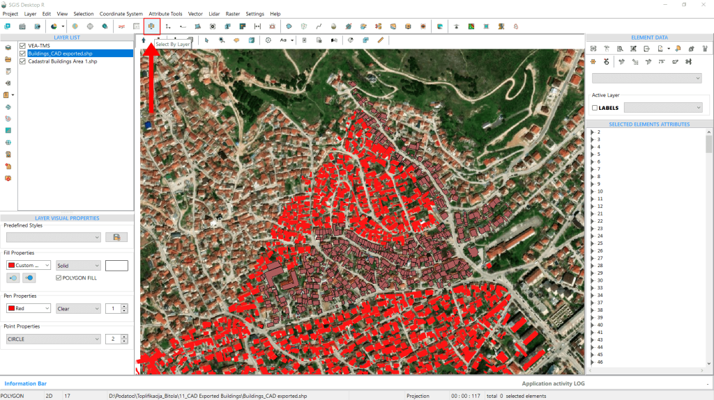
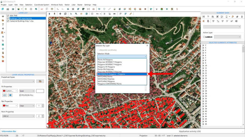
When the dialog window opens, we navigate to the ‘Selection Mode’ dropdown list, where we look for ‘Differences – Polygons with Polygons’. Once we find it, we click on it.
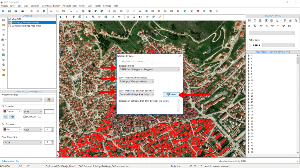
From the ‘Layer to be selected’ dropdown, we choose the Exported Building Footprints. Next, in the ‘Condition Layer’ dropdown, we select the Cadastral Building Polygons. Finally, we click on ‘Select’ to proceed.
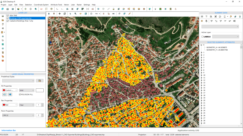
As we can see, the buildings that meet our criteria are instantly selected and highlighted in the graphics panel. Additionally, in the ‘Selected Elements’ panel, a tree-like list is created, displaying the attributes of each selected element. By clicking on an element in this list, its data becomes visible, allowing us to view specific area information without needing to open the attributes table.
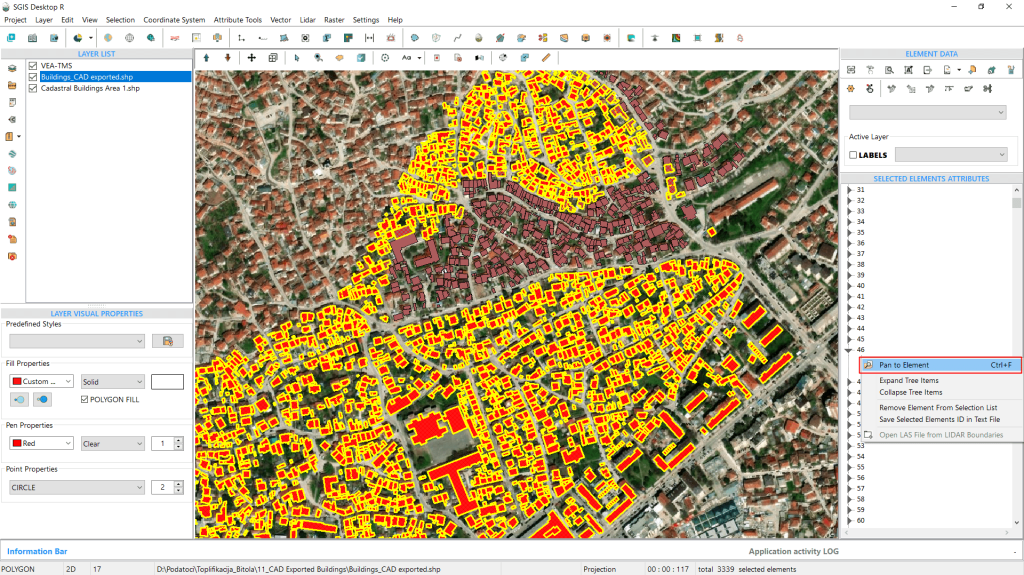
We can right-click on any element if we want to pan to a specific feature in the graphics window.
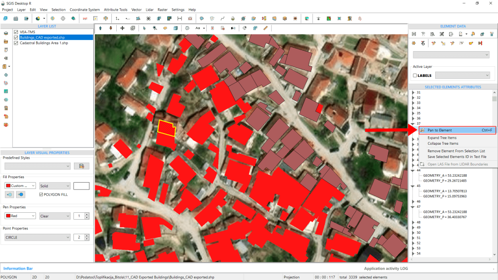
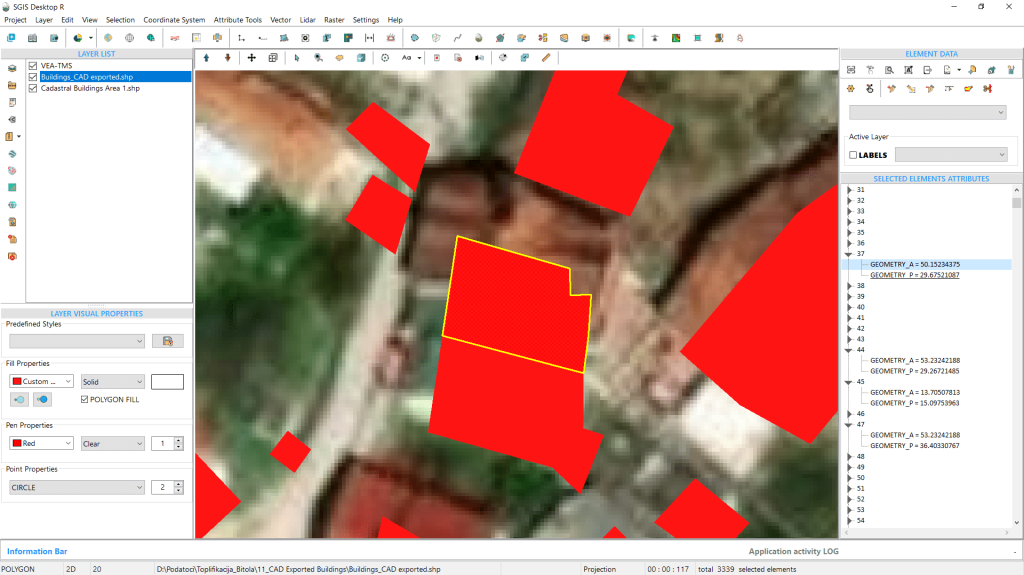
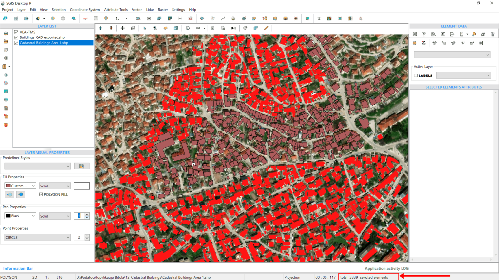
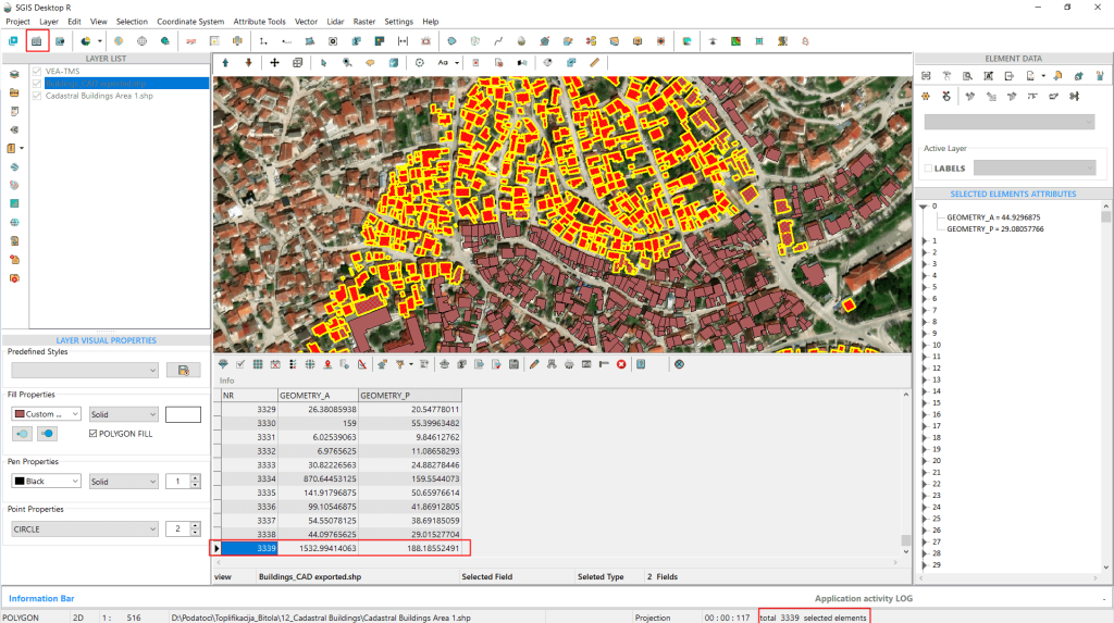
Another helpful feature that SGIS automatically provides is the total number of selected elements from the spatial selection process, even after the procedure is complete and turned off.
In the infobar, we can see that we have selected a total of 3,339 elements, or building polygons, in our example.
To verify this, we can repeat the selection procedure. While the selection is active and the buildings are highlighted, we can open the attribute table. From there, we can confirm that the exact same number of building polygons is displayed.
This concludes our procedure.
‘Matching Points’ is a spatial relationship criterion used in GIS to identify points in one dataset that correspond exactly with points in another dataset, based on their spatial location.
This criterion is used to find identical point features between two layers. Here, point features from two datasets are compared to determine if they share the same location.
This spatial analysis is used for identifying corresponding or duplicate points between layers, which can be essential for tasks like data validation, merging datasets, or ensuring data consistency.
One of the main uses of ‘Matching Points’ in GIS is data validation. When integrating datasets from different sources, you can use ‘Matching Points’ to check for duplication or consistency between the datasets. If points don’t match as expected, it could indicate errors in data collection or input.
Another key use is quality control. Users can use this criterion to ensure that point data from a newly surveyed dataset matches existing official data, such as matching new geospatial survey data to an existing cadastral layer or infrastructure dataset.
One more important use worth mentioning is data merging. If for example we’re working with multiple point datasets representing the same features (e.g., city street lights collected by different teams), ‘Matching Points’ allows you to combine the datasets, ensuring that duplicate entries are removed, and attributes are merged.
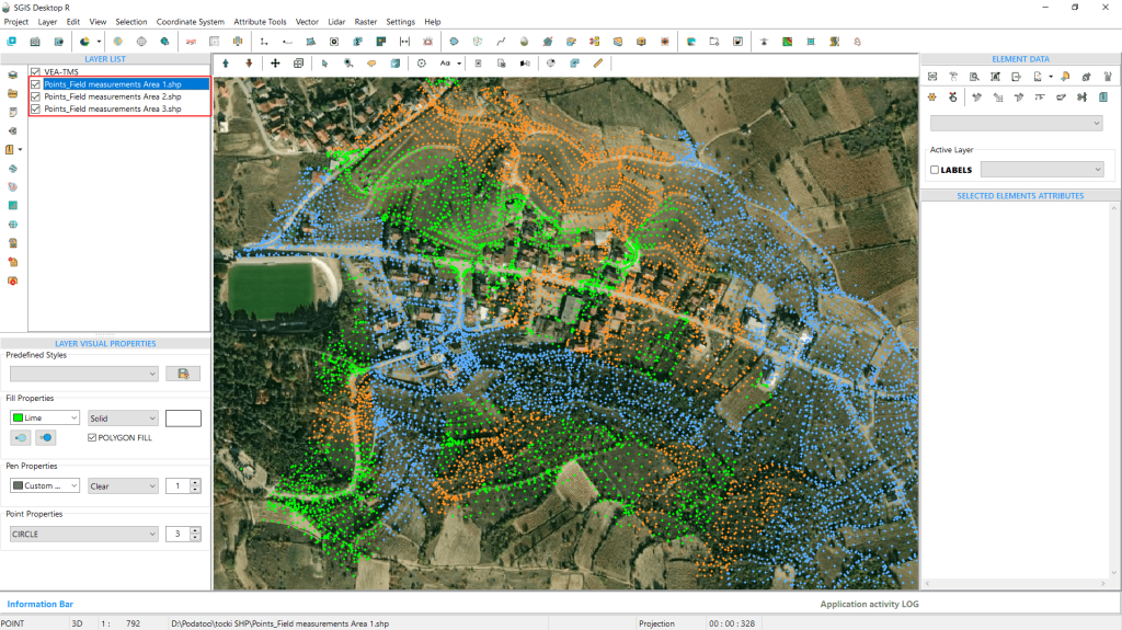
In this practical example, we’re working with three different datasets of land survey point data. We’ll use the Matching Points criterion to check for any duplicates across the datasets before merging them into one file. The first dataset is displayed in lime green on the graphics panel, the second in sepia, and the third in blue.
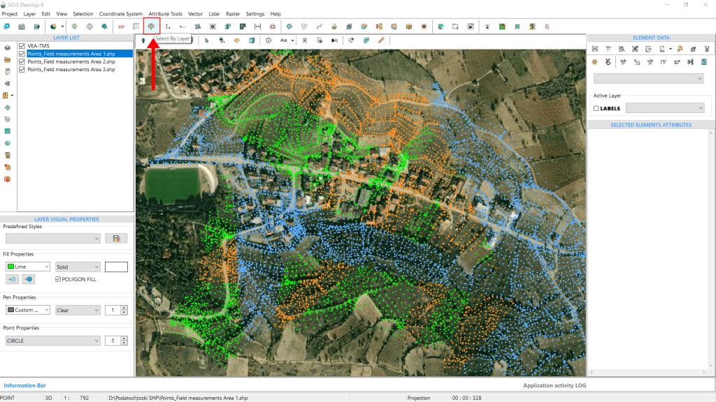
We’ll begin by using the ‘Select by Layer’ function.
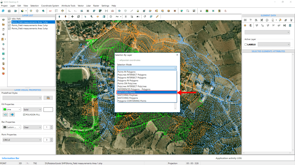
Next, select the ‘Matching Points’ option from the ‘Selection Mode’ dropdown list in the dialog window.
Then, from the second dropdown list labeled ‘Layer to be selected,’ we will choose the first measurement dataset, named Area 1.
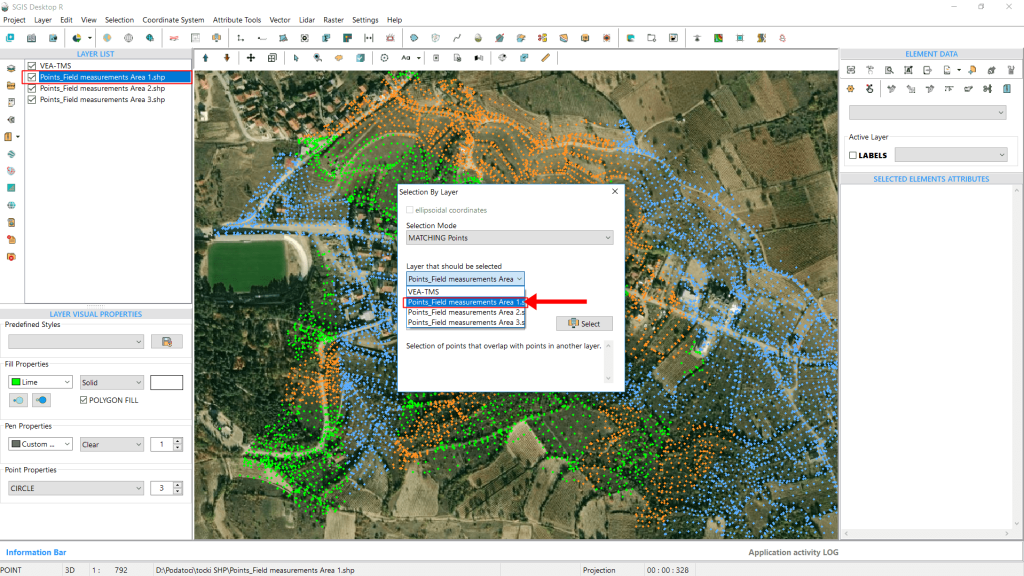
From the ‘Condition Layer’ dropdown, we’ll choose Area 2. This allows us to select and highlight all the points in Area 1 that are geometrically identical to those in Area 2, essentially identifying the duplicate points present in both layers. Once we have selected all the duplicates, we can either separate them into a new layer or delete them using the ‘Delete Elements’ tool.
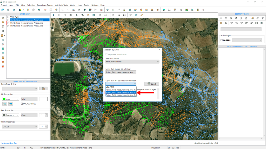
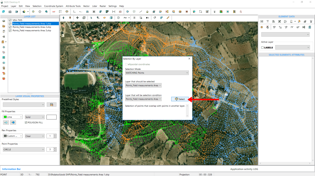
Next, we click on ‘Select’ to proceed.
The points are instantly selected and highlighted in bright yellow. It’s clear that many points overlap between Area 1 and Area 2. Next, we’ll clear the selection to see if there are also numerous matching points from Area 2 in Area 3.
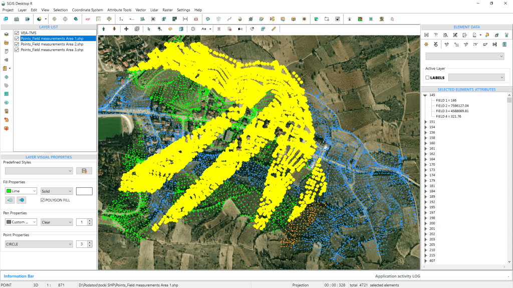
To clear the selection, we’ll head to the ‘Clear Selection List’ function found in the main toolbar of the user interface.
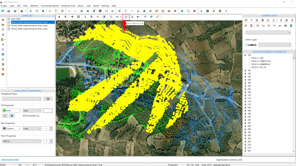
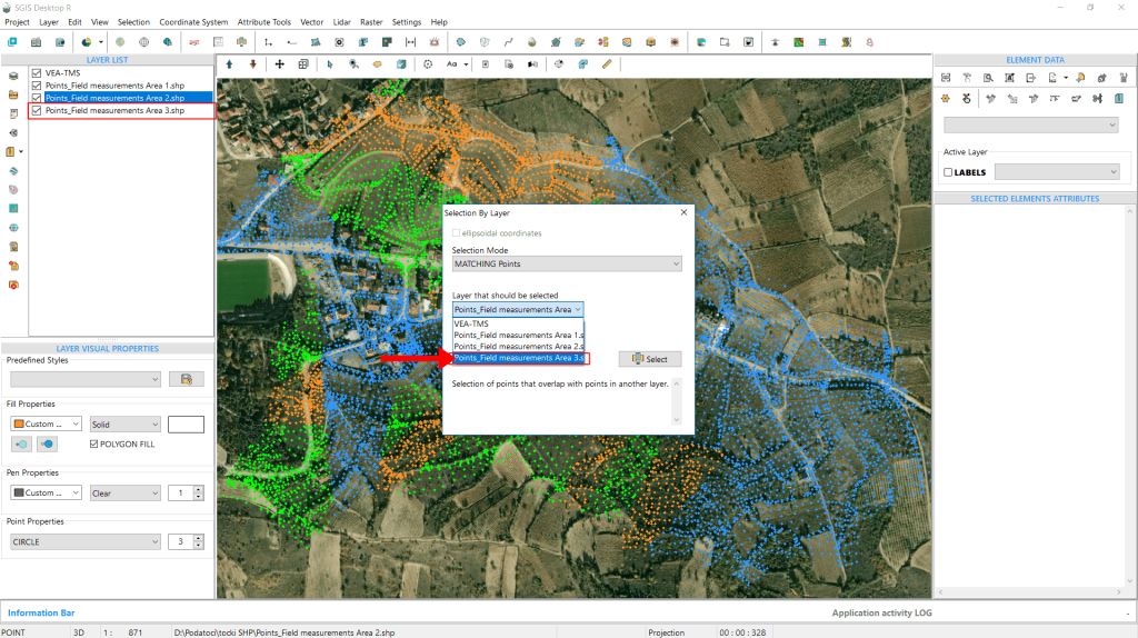
After deselecting the points, we’ll go through the procedure again and reopen the ‘Select by Layer’ dialog. We’ll keep the Selection Mode set to Matching Points. This time, we’ll change the selections for the ‘Layer to be selected’ and the ‘Condition Layer.’ From the ‘Layer to be selected’ dropdown, we’ll choose the measured points labeled as Area 3.
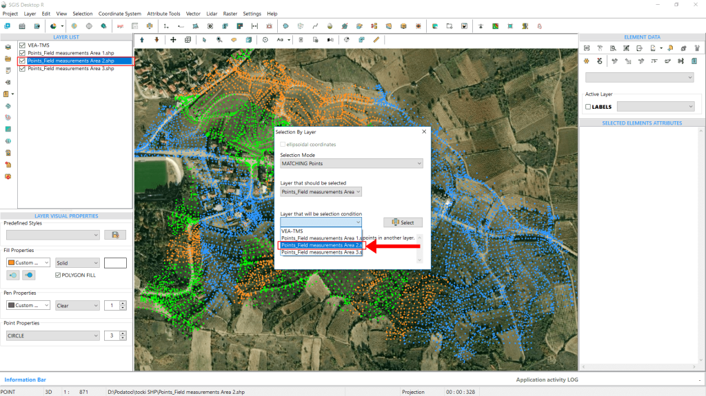
This time, we’ll choose Area 2 from the ‘Condition Layer’ dropdown list.
Once again, we click on ‘Select’ to start the process.
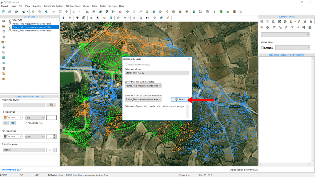
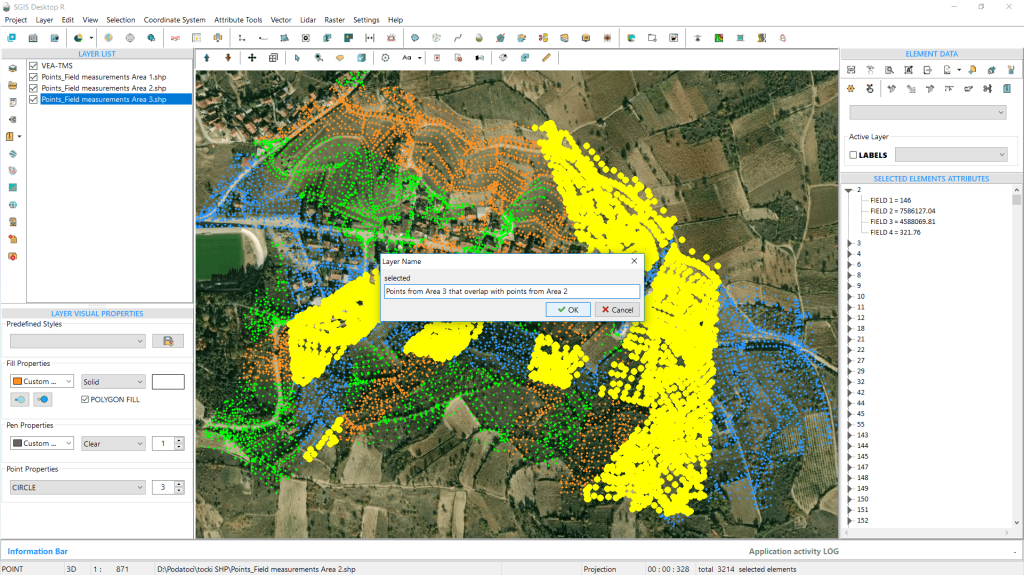
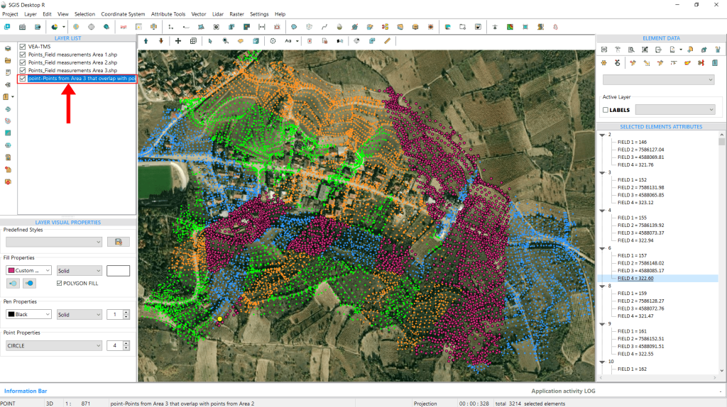
We can now see the set of matching points, which are points from Area 3 that coincide with those from Area 2. To illustrate the function, we’ll isolate these points into a separate layer. This will allow us to export them later and continue with our work, as we are still waiting for a few more datasets from the land surveyors.
These points will eventually be used to produce contour lines for the terrain, and once we have all the datasets collected and complete, we’ll merge them into one comprehensive file.
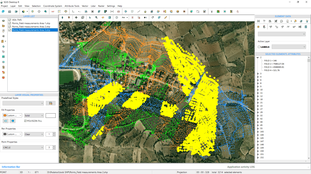
For now, let’s proceed with the ‘Selected Elements in New Layer’ function. We’ll name the newly created layer and click ‘OK.’ The new layer will appear instantly in the Layers panel.
If someone wishes to delete the selected points—since they already exist in the other layer (Area 2)—they can easily do this by clicking the ‘Delete Element’ function in the ‘Element Data’ panel. Since all the points are selected, they will be deleted at once.
With that, we’ll conclude our procedure.
The ‘Matching Polylines’ spatial relationship criterion refers to identifying polylines in one dataset that exactly correspond with polylines in another dataset within a GIS environment, based on their spatial geometry or location. This criterion helps in identifying identical line features between the two layers.
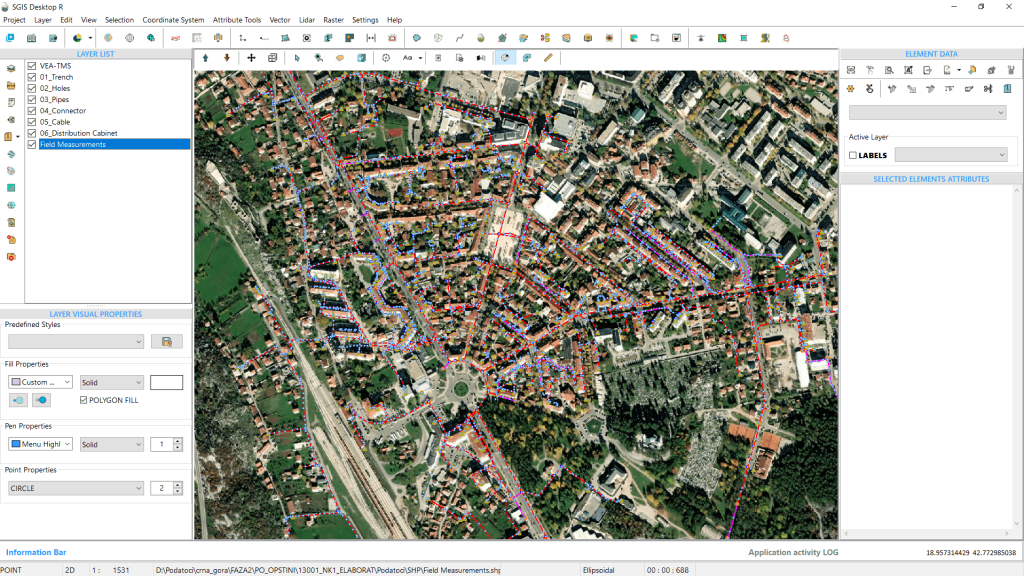
In our ninth practical example, we’ll be working with a telecommunications network that includes various infrastructure elements such as manholes, pipes, distribution cabinets, connectors, trench lines, and optical cables.
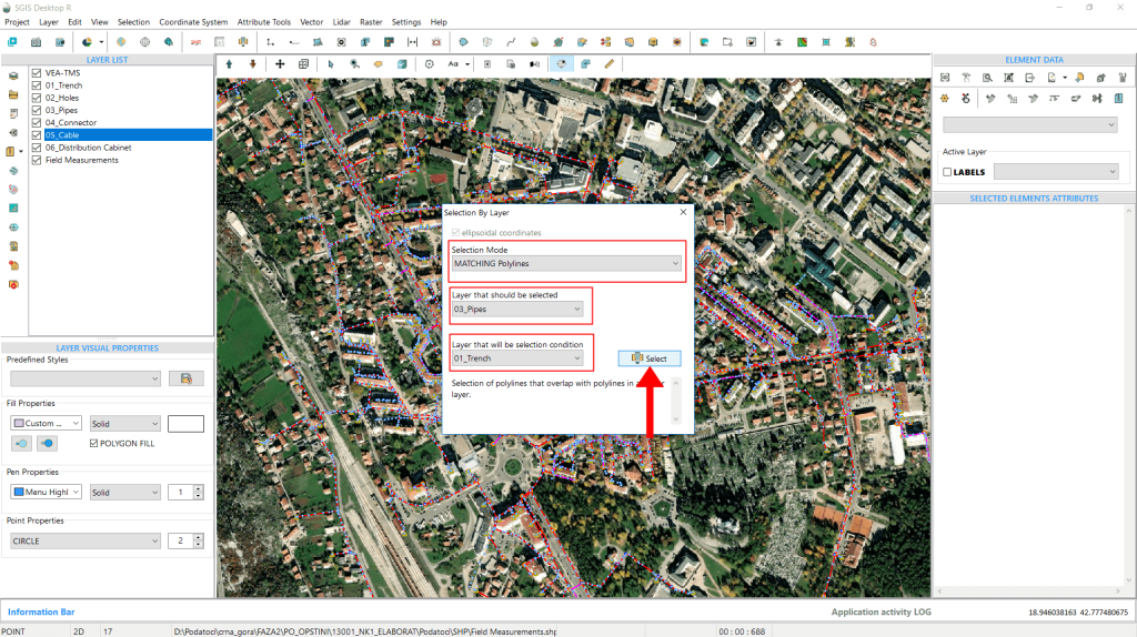
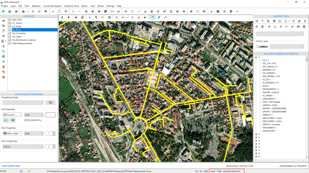
Given the multiple layers and datasets involved, we want to select all the telecommunication cables that are located inside the designated pipes. Additionally, we want to identify where underground pipes have already been placed along the trench lines.
Let’s get started.
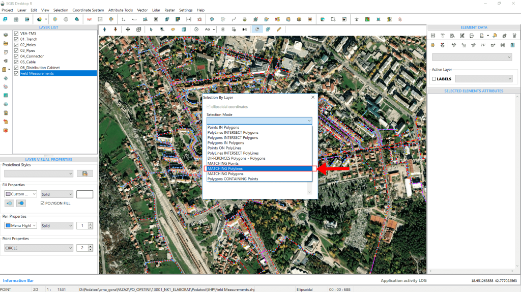
We’ve added a basemap in the background for better visual clarity. Now, let’s proceed by opening the ‘Select by Layer’ function. First, we navigate to the dropdown menu and choose the ‘Matching Polylines’ option for the Selection Mode.
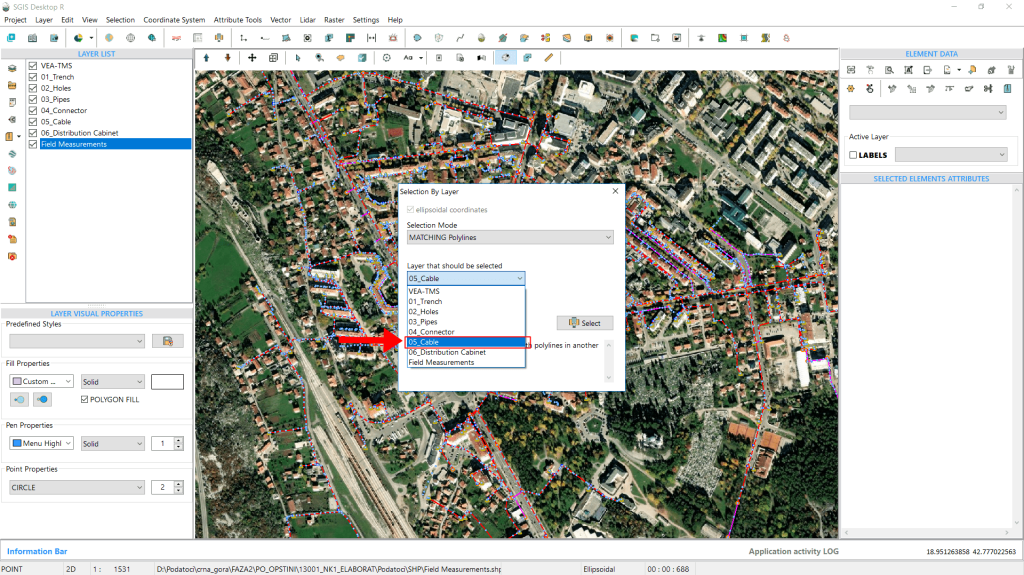
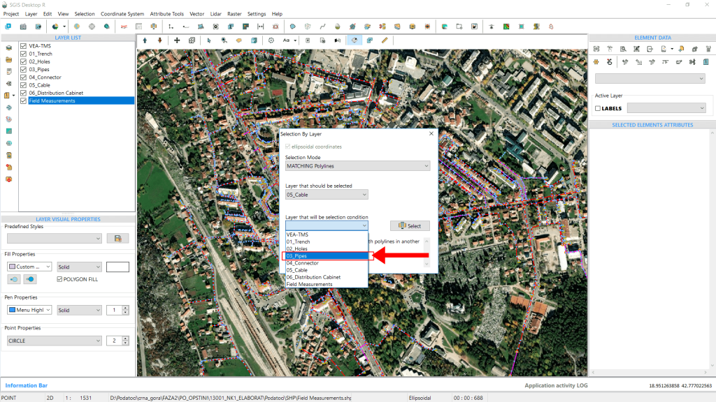
Next, from the second dropdown, we select the layer containing the features we want to highlight— in this case, the ‘Cable’ layer. Then, from the third dropdown, which sets the condition layer, we select the ‘Pipes’ layer to define the selection criteria.
Finally, we click ‘Select’ to run the process.
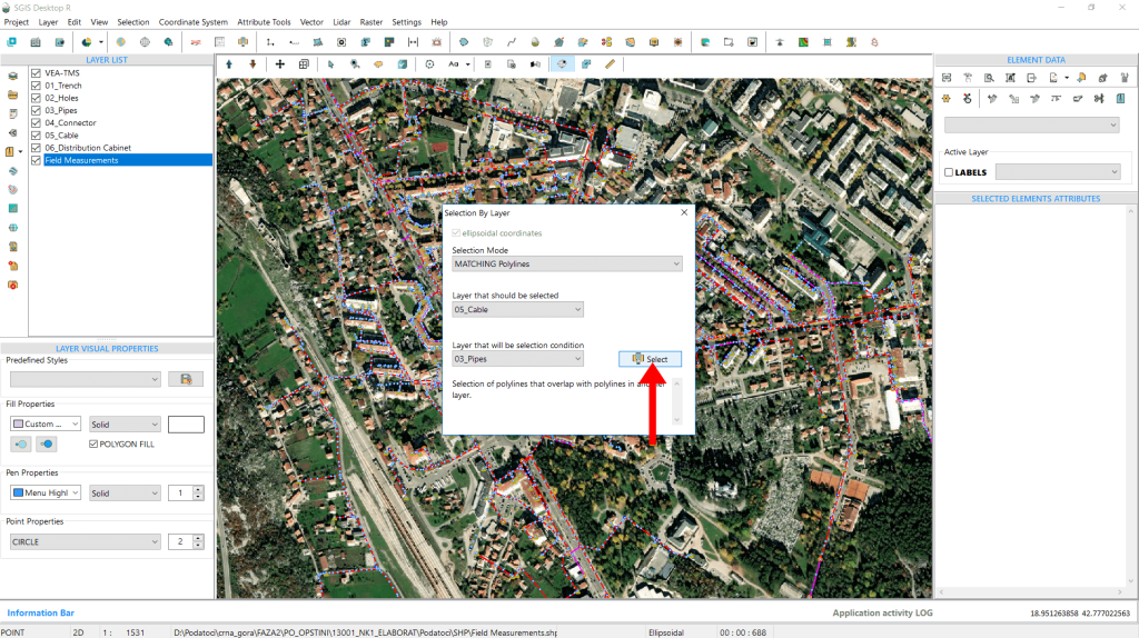
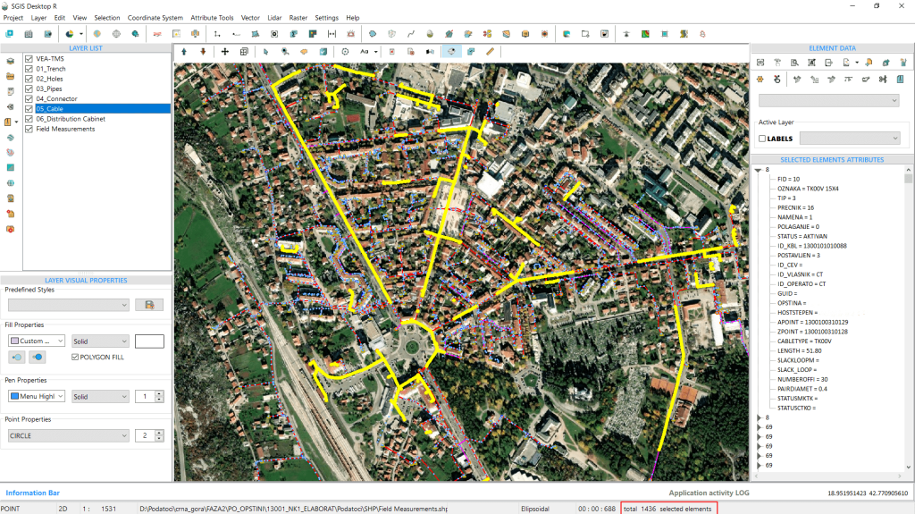
As shown in Fig.104, the optical cable network is highlighted, indicating the pipes it runs through. From this selection, users can isolate the cable elements and add additional attributes, create a new layer, or use the ‘Selected Elements’ panel to review and manage specific elements without opening the full attributes table. The attributes table also offers additional options for previewing elements on the graphics panel window based on specific attribute field conditions, but we’ll explain that in another use case documentation.
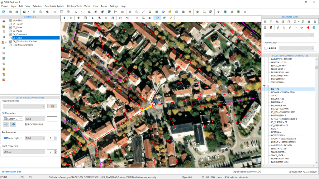
We’ll go through the process once more to assess the progress of the fieldwork by checking the placement of the pipes along the underground trench line. This will give us insight into how much work the construction team has completed. To do this, we need to select all the pipes that correspond to the trench layer. So, let’s click on ‘Select’ to begin.
And with that, we’ve completed our selection procedure.
The ‘Matching Polygons’ spatial criterion in GIS is used to identify polygons from one dataset that match polygons in another, typically based on their spatial geometry or location. In SGIS, both in Desktop and v.R versions, this criterion focuses on the precise geometric properties of the datasets. When searching for matching features, the algorithm checks for polygons that do not exceed a tolerance of 0.02 meters (2 cm) in length between them. Additionally, the vertices that make up these polygons must align exactly for the match to be valid.
This feature is especially valuable in sectors like cadastral mapping, land administration, and urban planning, as it allows for efficient management of large-scale projects where precision is critical for both legal and practical purposes.
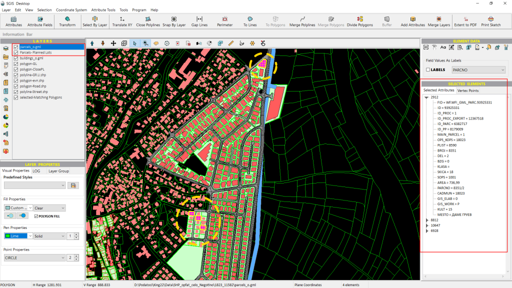
In our practical example, we’ll demonstrate this by using the ‘Matching Polygons’ criterion to compare a cadastral dataset with polygonal footprints representing urban parcels. These parcels are designated for residential use, and in addition to them, we have data on streets and buildings. Our goal will be to identify how many of these urban residential parcels exactly match or coincide with the official cadastral boundaries. Let’s dive in!
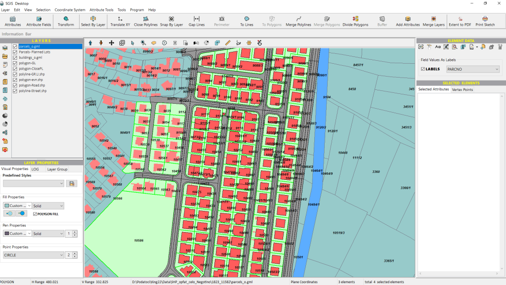
Once all the data has been imported, we’ll go to the ‘Select by Layer’ function.
From the Selection Mode dropdown menu, we’ll choose the ‘Matching Polygons’ option.
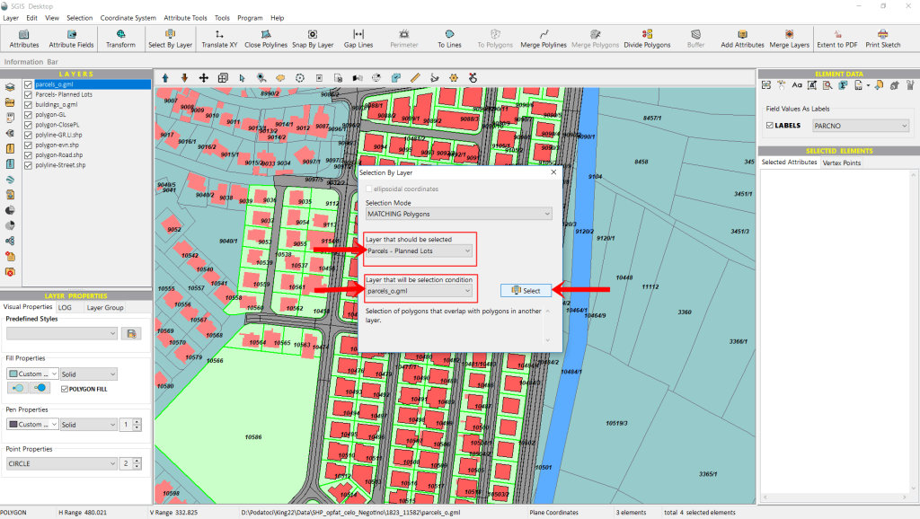
Next, under the ‘Layer to be selected’ dropdown, we’ll select the Urban parcels layer, as we want to highlight parcels from this dataset.
The Cadastral parcels layer will act as the condition layer for this selection.
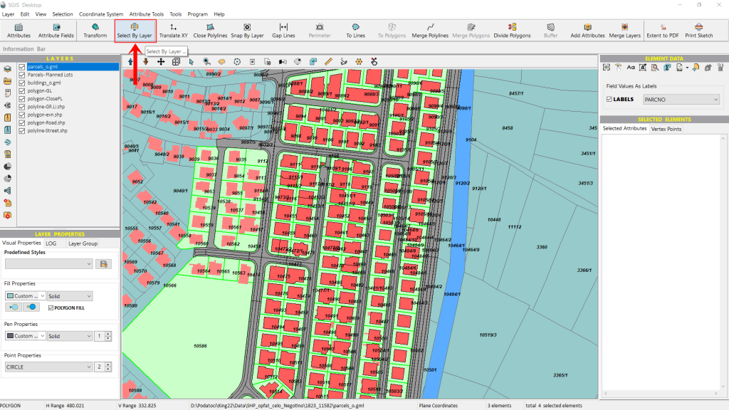
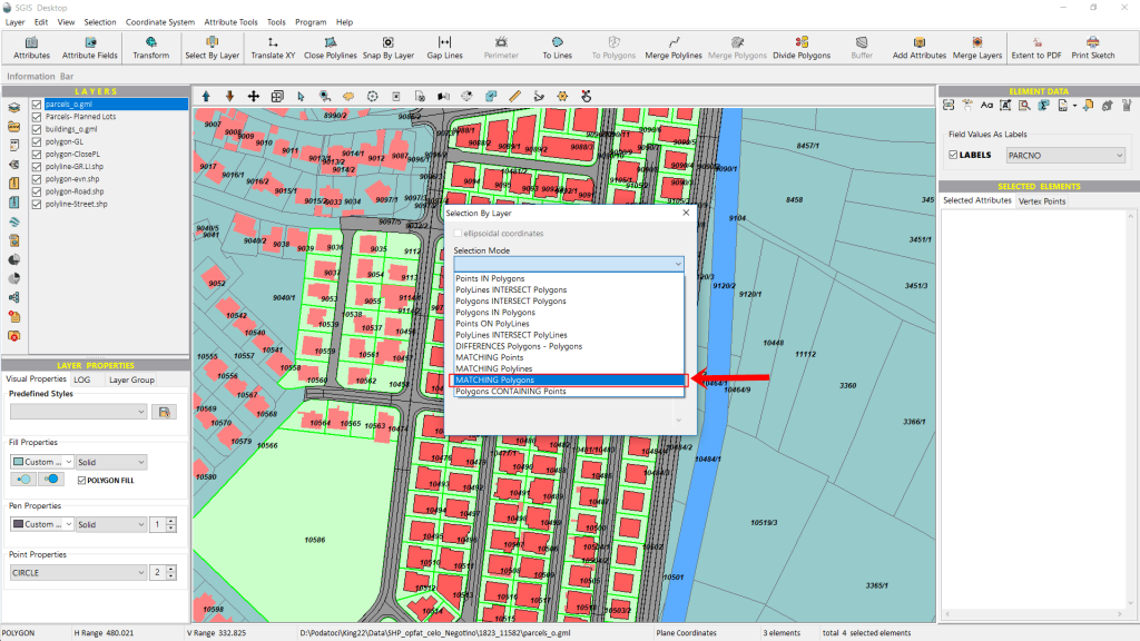
From the condition layer dropdown, we’ll select the Cadastral Parcels layer.
As mentioned earlier, it’s important to note that the algorithm has a default tolerance of 0.02 meters. Additionally, the matching process will only recognize polygons as identical if they have the exact same number of vertices—any difference in vertex count will disqualify them from being considered a match.
Once all the layers are set, simply click ‘Select’ to begin the process.
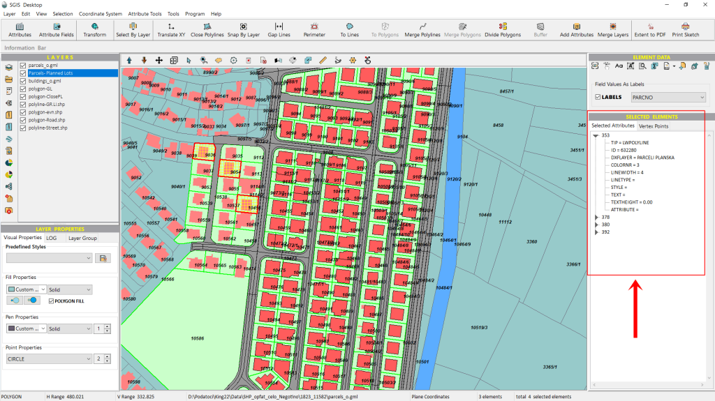
As shown in Fig.112, the polygons that meet the matching criteria are highlighted on the graphics panel.
Additionally, the selected elements are listed in the ‘Selected Elements’ panel in a tree-like structure. Since the list shows four elements, but only three are visible on the graphics panel, we’ll select the first item in the list, right-click on it, and use the ‘Pan to Element’ function to locate it on the map.
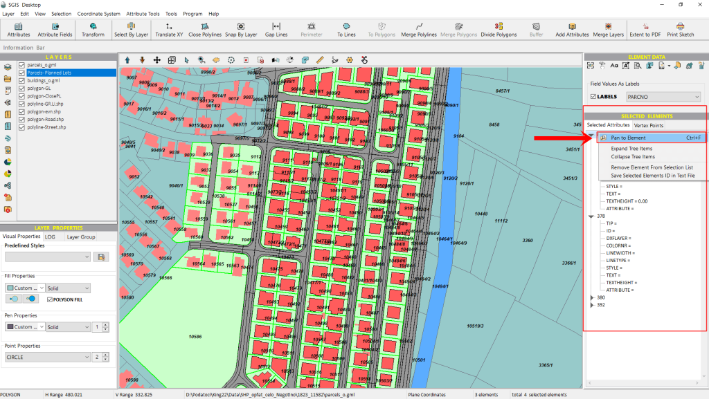
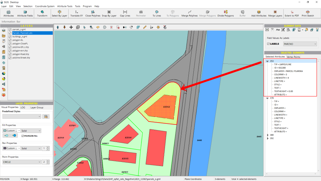
Immediately, the first element is highlighted on the graphics panel, offering better visual clarity regarding its geometry and location.
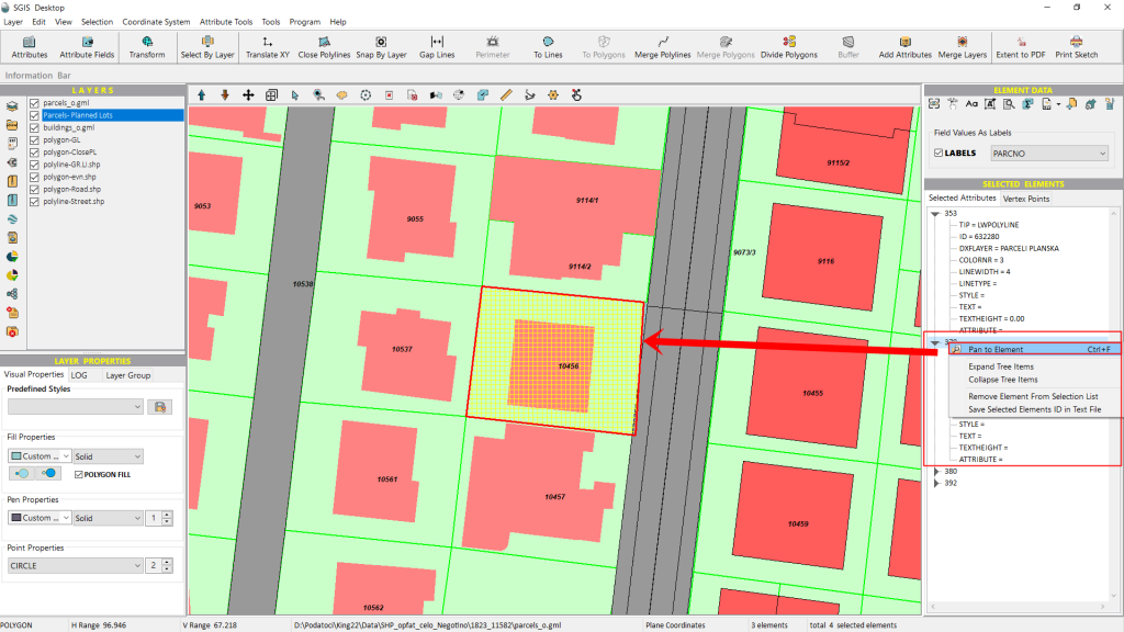
Next, we’ll select the second element from the ‘Selected Elements’ list and right-click on it to pan to that element as well.
Next, we’ll separate the selected urban parcels into a new layer.
After that, we’ll switch to CAD mode to continue editing the data.
This will bring our procedure to a close.
The ‘Polygons Containing Points’ spatial criterion is used to select polygons that contain specific points within them. This criterion is highly valuable in GIS for several reasons;
It allows users to analyze the spatial relationships between different geographic features, such as identifying which areas (polygons) include particular locations (points). This is particularly useful in applications like land-use analysis, resource management, and urban planning.
It also helps in linking point data—such as population centers, sensor locations, or incidents—to larger geographic areas like administrative zones, land parcels, or ecosystems. This is beneficial for demographic studies, service coverage analysis, and environmental monitoring.
In cadastral mapping and infrastructure projects, it ensures that point features, such as infrastructure nodes, are accurately positioned within their designated areas (polygons), supporting spatial data accuracy.
In our practical example, we’ll be working with infrastructure point data overlaid on a designated polygon area, representing a specific telecommunication zone. This entire network is connected to one particular distribution cabinet, illustrating how this criterion helps manage and analyze complex network systems.
We need to evaluate which street numbers, represented by points in the street number layer across all zones, fall within Zone 1. Additionally, Zone 1 is divided into several polygon areas, so we’ll be assessing which specific polygons contain which points.
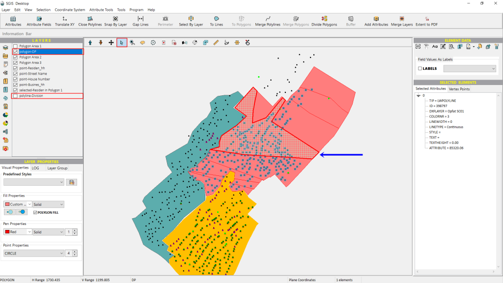
In practice, we begin this process using the ‘Polygons Containing Points’ selection mode and then finalize it with the ‘Points in Polygons’ mode. However, since we are demonstrating only one function here, our focus will be on the ‘Polygons Containing Points’ selection mode. For this example, we’ll wrap up with that. A complete guide, covering multiple procedures from start to finish, will be available in more in-depth case studies.
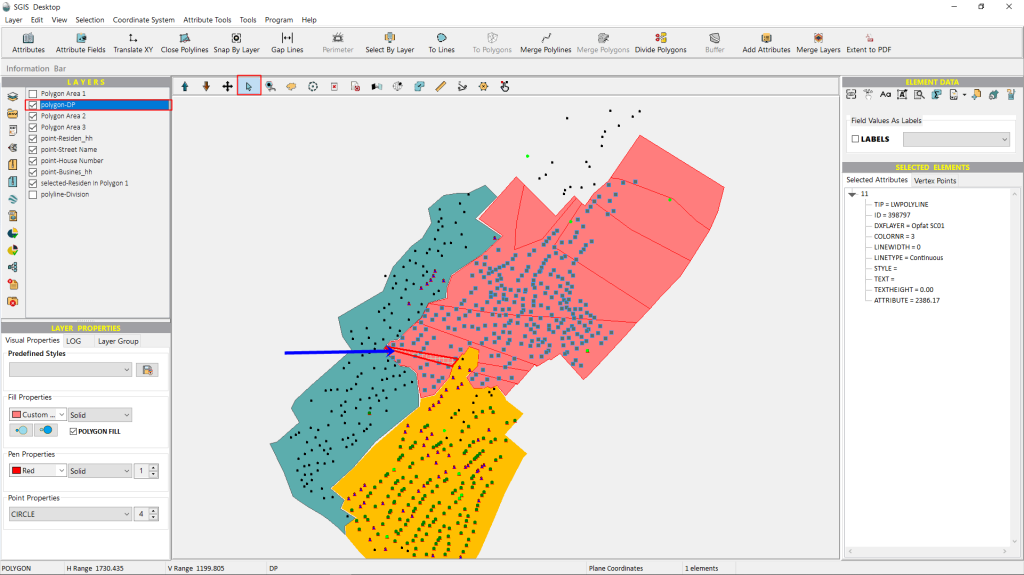
Zone 1 consists of several distinct areas, and for demonstration purposes, we’ll select just one polygon feature.
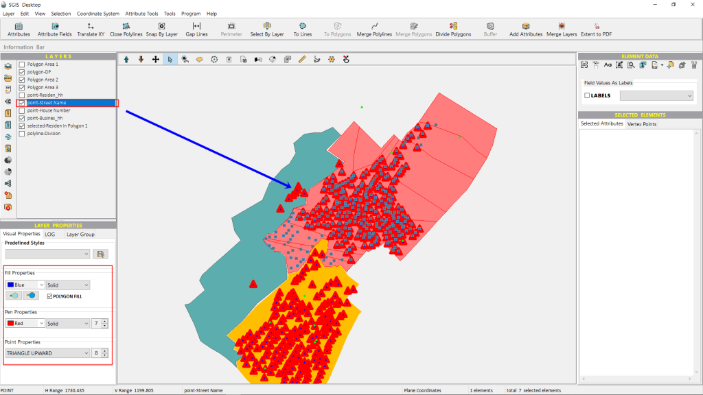
Before we begin the selection process, let’s adjust the visual properties of the Street Number layer. We’ll change the points to upward-facing red triangles. This adjustment will help differentiate the various point layers, making it easier for users to see and understand the data more clearly.
Next, we’ll set the selection mode to ‘Polygons Containing Points.’ The layer to be selected is ‘polygon-DP,’ which stands for Divided Parcels and contains all the parcels within Zone 1. For the condition layer, we’ll choose ‘Street Name,’ a point layer that holds all the street name points for the three zone areas.
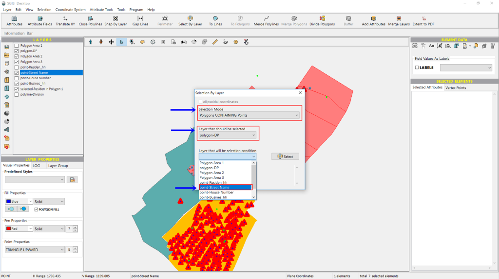
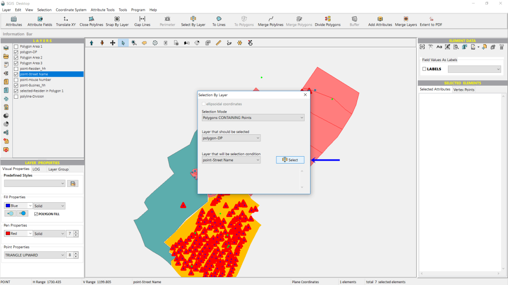
We click on ‘Select’ to initiate the selection process.
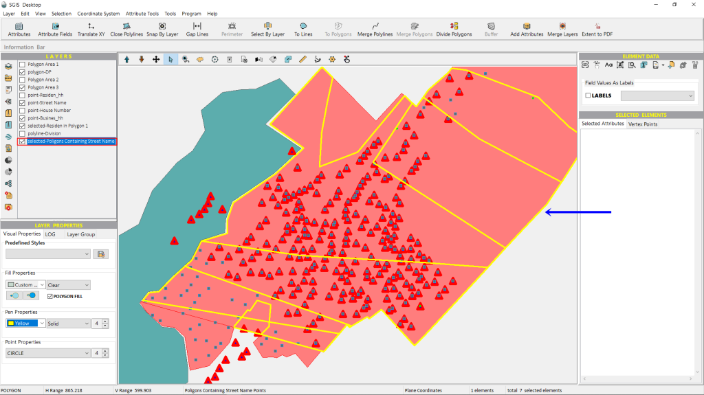
The polygons within Zone 1 that meet the specified criteria are immediately highlighted and selected. As shown in Fig.122, five polygons in Zone 1 do not contain any street name points, while seven polygon features have been successfully selected.
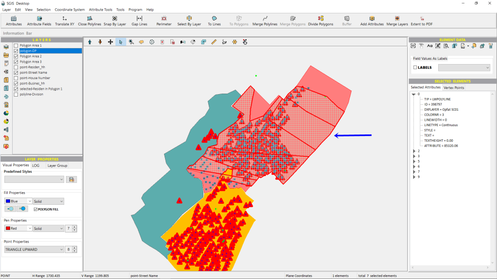
We’ll use the ‘Selected Elements in New Layer’ function to isolate these 7 selected polygons into a new, separate layer.
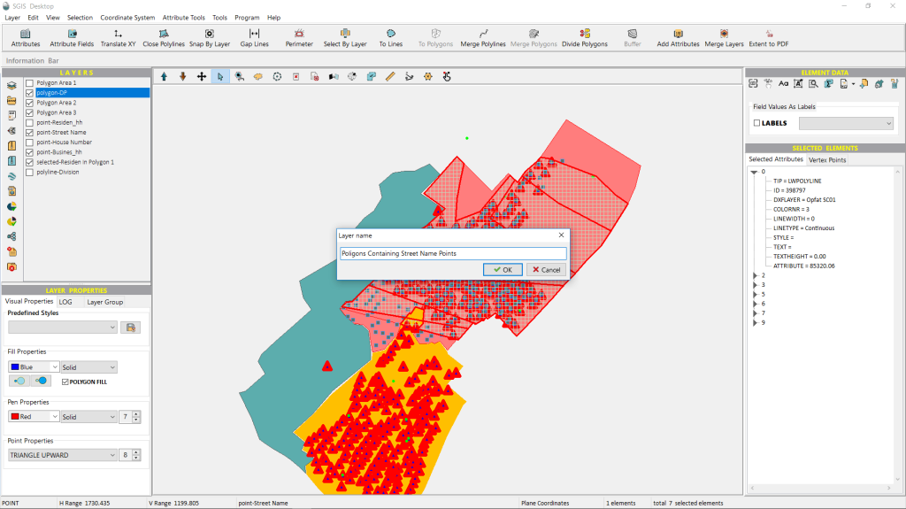
The new layer is created and displayed with yellow polygon boundaries in a no-fill style, making the data we want to focus on easier to see.
With this step, we conclude our selection process.