
The LAS file format versions (LAS 1.1, LAS 1.2, LAS 1.3, and LAS 1.4) represent different revisions of the LAS specification, each introducing new features and improvements to accommodate the evolving needs of LiDAR data storage and usage. These versions are maintained by the American Society for Photogrammetry and Remote Sensing (ASPRS).
Version Numbers and Specification Dates:
- LAS 1.1: Introduced in 2005.
- LAS 1.2: Introduced in 2008.
- LAS 1.3: Introduced in 2009.
- LAS 1.4: Introduced in 2011 with a revision date of March 26, 2019.
The LAS format consists of binary data in little-endian format, structured into:
- Public Header Block
- Variable Length Records
- Point Data (for LAS 1.1, LAS 1.2, and LAS 1.3)
LAS 1.4 introduces an additional component:
- Extended Variable Length Records
Point Data Record Formats:
For LAS 1.1, LAS 1.2, and LAS 1.3:
- Point Data Record Format 0
- Point Data Record Format 1
- Point Data Record Format 2
- Point Data Record Format 3
- Point Data Record Format 4
- Point Data Record Format 5
For LAS 1.4, additional formats are included:
- Point Data Record Format 0
- Point Data Record Format 1
- Point Data Record Format 2
- Point Data Record Format 3
- Point Data Record Format 4
- Point Data Record Format 5
- Point Data Record Format 6
- Point Data Record Format 7
- Point Data Record Format 8
- Point Data Record Format 9
- Point Data Record Format 10
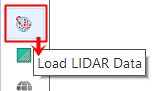
To demonstrate how SGIS v.R supports LAS formats, including LAS 1.1, 1.2, 1.3, and 1.4, simply click on the ‘Load LIDAR data’ function. This simple step will let you work with different versions of LAS files, making the process both straightforward and user-friendly within the software.
Let’s start with the real-world example:

To load the LAS file, start by opening the ‘Load LIDAR data’ function. You’ll find this function conveniently located in the ‘Open Data’ ribbon toolbox on the left side of the Layers Panel. You can also access it from the Layers tab in the main menu.

Once activated, a new dialog window will appear, where you’ll need to navigate to the file’s location path and select the file.
After selecting the file, click ‘Ok’ and wait a few seconds for it to load.
Once the import is complete, you’ll see a set of details about the file displayed in the info box below the ‘Open LAS’ button, providing you with key information about the file you’ve just opened.


The LAS file has been successfully loaded. To enhance visualization and improve location clarity, we’ve added a basemap overlay. With this, the loading procedure is complete, and the process is finished.
Classifications in LiDAR point cloud data play a crucial role in distinguishing various surface features, such as the ground, vegetation, buildings, or water bodies. By assigning classification codes to each point, users can easily differentiate objects within the landscape. This is especially important for tasks like generating digital elevation models (DEMs), monitoring vegetation health, analyzing urban infrastructure, and executing planning efforts in GIS environments.
With tools that allow users to manage these classifications, it becomes possible to filter and extract specific features, like isolating ground points for terrain modeling or excluding vegetation for urban planning. Proper classification ensures that subsequent analyses are more accurate and reliable. Moreover, classifications enhance visual representation, allowing different features to be displayed with unique colors or layers, simplifying data interpretation and communication.
SGIS v.R includes a built-in tool designed to help users manage classifications within a LiDAR point cloud. To access this tool, you’ll need to first ensure that a LAS file has been imported into the Layers List. Once the tool is ready, it can be opened with a single click. You can find it conveniently located in the ‘Element Data’ toolbox on the main interface, making it easy to manage and adjust classifications as needed.
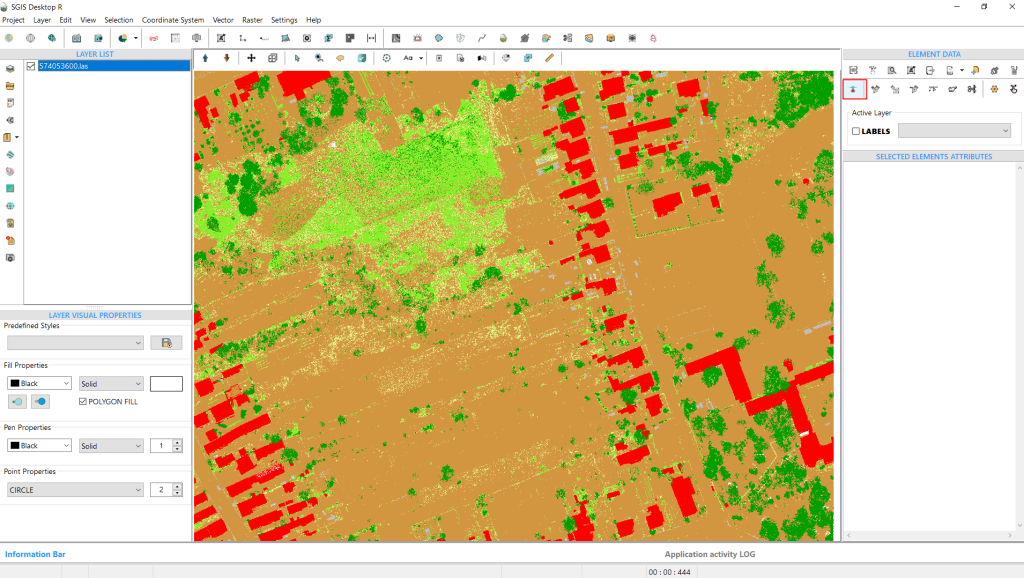
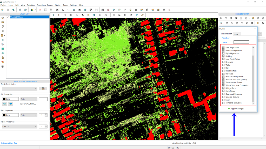
The function opens a new window with two tabs: ‘Classification’ and ‘Tools’. The ‘Classification’ tab opens by default. In this tab, users can view the Classification Number, Classification Color, and a list of classification codes. Each lidar point is assigned a classification that indicates the type of object reflecting the laser pulse. Lidar points can be categorized into various classes, such as ground, vegetation, buildings, or water. These classes are represented by numeric integer codes, which follow ASPRS standards for LAS formats 1.1, 1.2, 1.3, and 1.4. All ASPRS-defined classification codes are listed in the toolbox window, with all options checked by default.
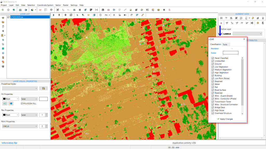

Users can easily control which class codes are visible by checking or unchecking the desired classifications. In the example shown, we’ve unchecked classification codes 1 and 2, representing unclassified points and ground points.
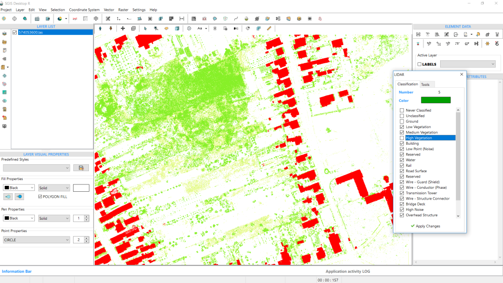
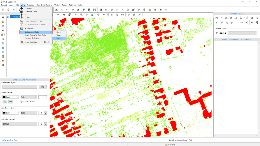
If you want to uncheck more classification codes and work with just a few, but find the graphics panel too bright, you can use the ‘Change Background Color’ function. This option is located in the View toolbar in the main Menu.
You can choose from three background colors: white, silver, and black. For this example, we’ll select black. Once clicked, the graphics panel will change instantly.
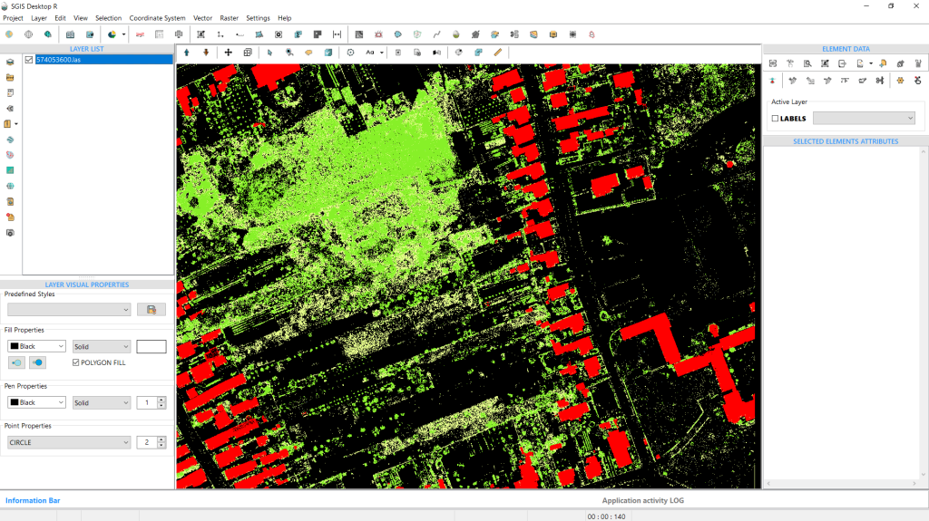
Now, moving on to the LIDAR toolbox. As mentioned earlier, all classification codes are listed and checked by default. However, the point cloud in our example doesn’t include points for every classification code. Only a few of the available codes in the list are actually present in this point cloud.
Instead of unchecking each classification one by one, we can save time by switching to the second tab, ‘Tools’. Here, you’ll find a memo box with three distinct function buttons below it. The first button, ‘Get existing classification numbers,’ displays all the existing classification codes in the memo box in a clear, notepad-like format. Let’s click it to proceed.
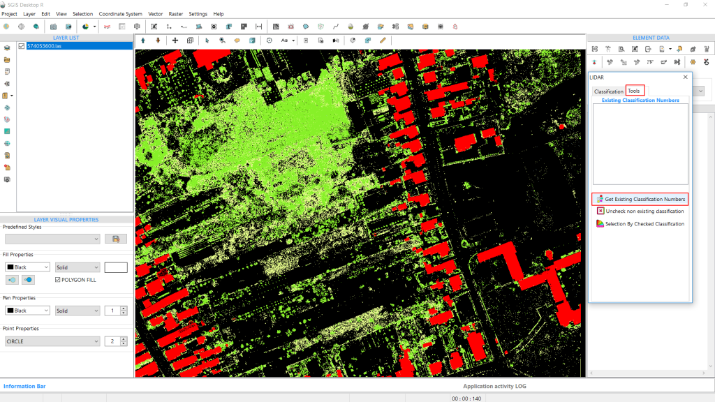
All classification codes that contain points are immediately listed in a column within the memo box.
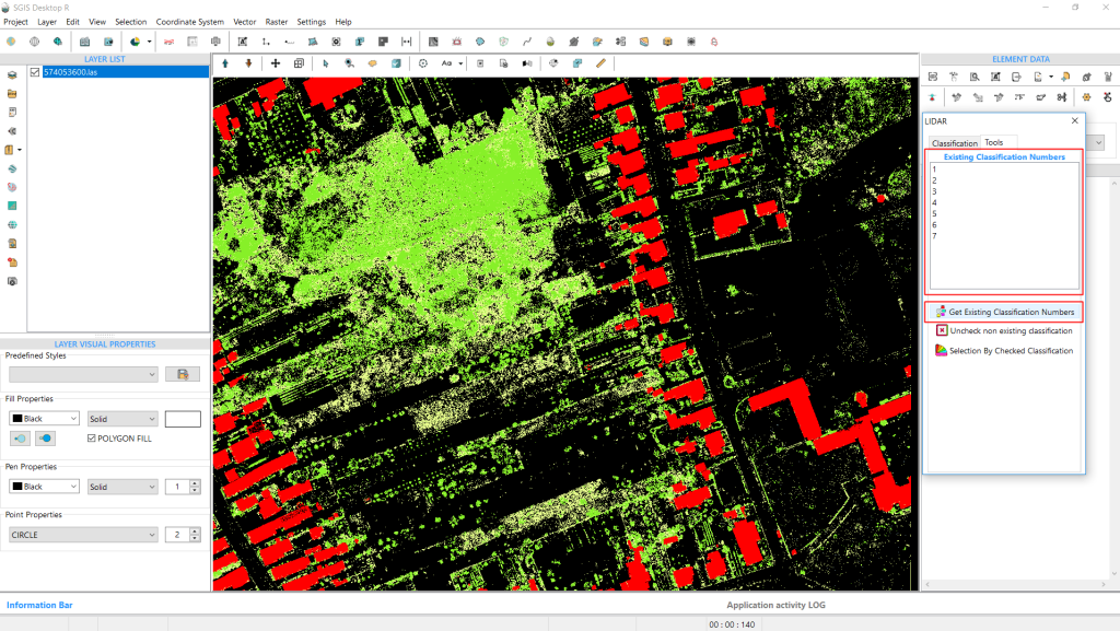
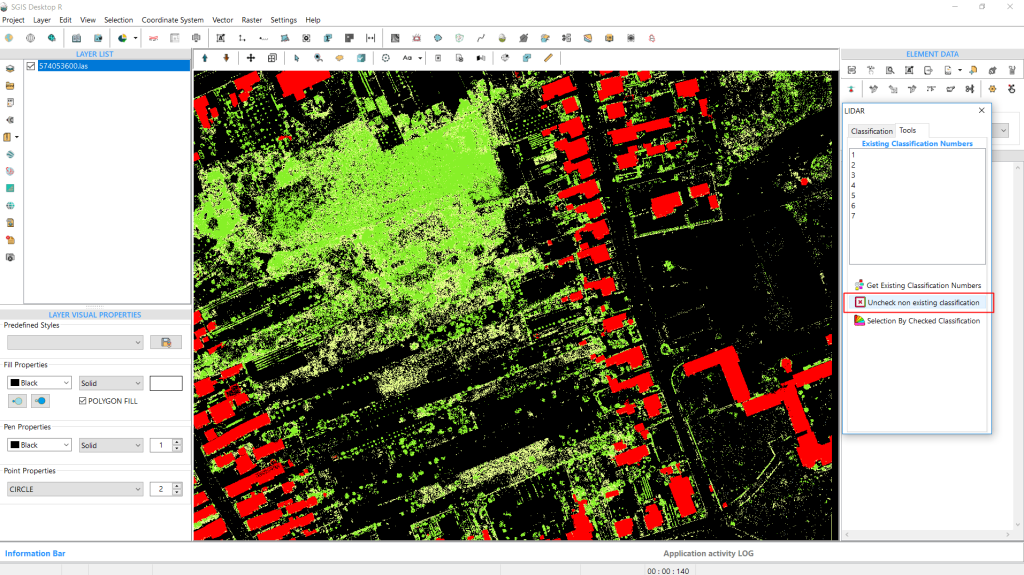
Below the ‘Get existing classification numbers’ button is another function called ‘Uncheck non-existing classification’. When clicked, it automatically unchecks all classification code layers that don’t contain points. Let’s go ahead and click it.
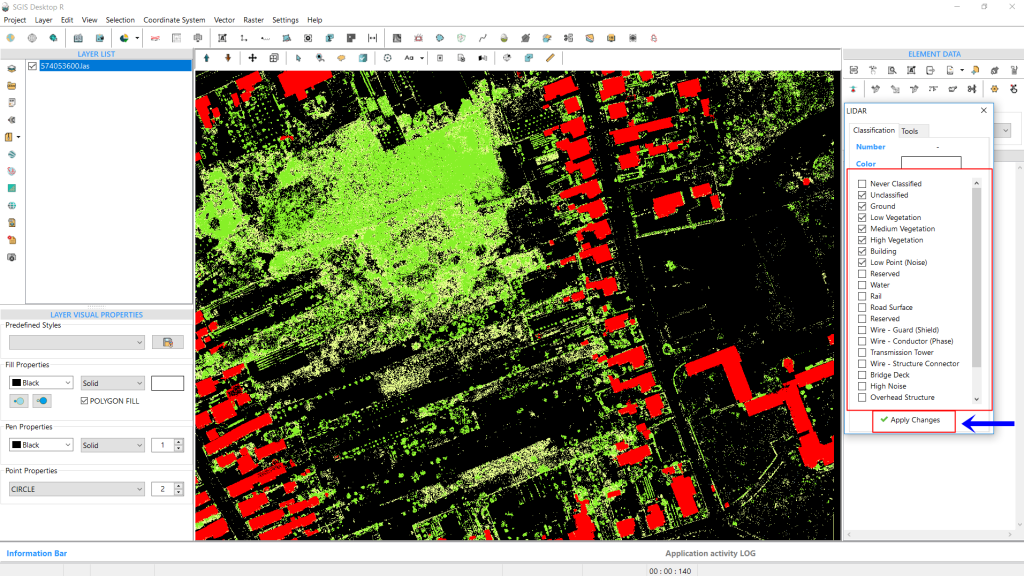
To apply the changes to the graphics panel, return to the ‘Classifications’ tab and click the ‘Apply Changes’ button. This will update the graphics panel with the new settings, completing the procedure.
Tailoring colors for different classifications improves the visual distinction between features such as ground, vegetation, buildings, and water, making the data easier to interpret. Additionally, projects may require a focus on certain features, and customizing colors allows users to emphasize the most relevant classifications for tasks like infrastructure planning or environmental analysis. This also ensures consistency across teams or projects, standardizing how the data is viewed and interpreted.
When importing a LiDAR point cloud into SGIS v.R, users can select the ‘Import with LiDAR Classifications’ checkbox. This imports the ASPRS classification list, which is pre-colored based on the defined classification values. Later, the ‘LIDAR’ tool allows users to customize the color of each classification, tailoring it to fit the needs of their specific project.
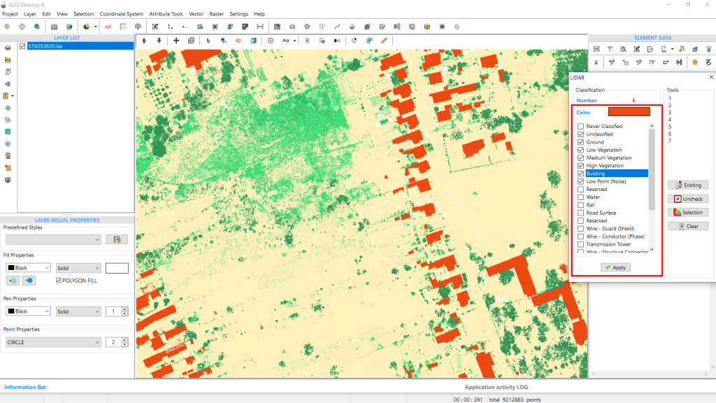
To begin customizing the colors for each class, users can open the LiDAR toolbox. In the Classifications tab, under “Number,” there is an option labeled “Color.” Next to it, a colored rectangle displays the current color of the class. This rectangle is clickable, and clicking on it opens a color palette. Users can either select a color from the palette or input specific RGB or HSL values.
For this demonstration, we’ll assign different colors to the classifications in our point cloud. Starting with the 2nd class, which represents the ground, we’ll change the color for each existing class. In the end, the point cloud will be uniquely colored, tailored to the specifications of our project.
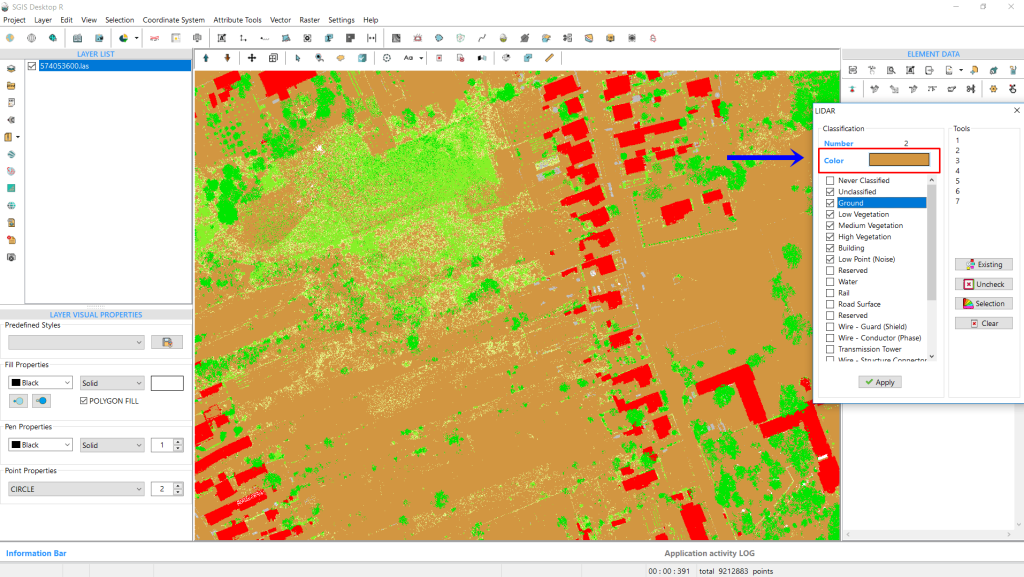
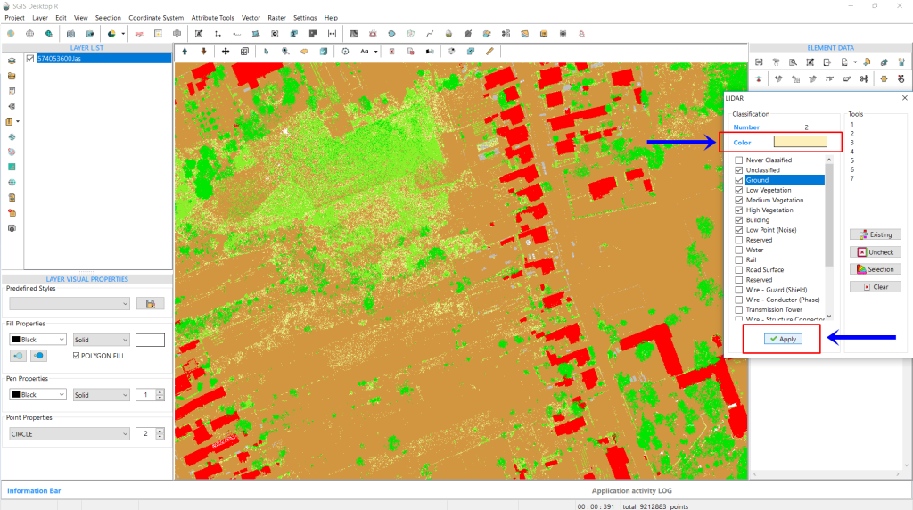
After adjusting the colors, it’s necessary to click ‘Apply’ for the changes to take effect and become visible in the graphics panel window.
The changes have been applied, and with that, the procedure is complete.
Creating separate GIS layers from a LiDAR dataset allows for tailored visualization. For instance, you can use different color schemes or styles to highlight vegetation in one layer and other features in separate layers. Isolating the ground class, for example, enables focused analysis of terrain and surface features, which is essential for tasks like topographic mapping and terrain modeling. Separating the buildings class allows for detailed examination of urban structures, crucial for city planning, infrastructure development, and property management. Overall, isolating different classes into separate GIS layers enhances data management and supports more precise and effective analysis.
SGIS enables these modifications using the ‘LIDAR’ toolbox.
We previously loaded a point cloud into SGIS v.R. Opening the ‘Lidar’ toolbox reveals a dialog window where we have already seen how to populate the memo box with existing classification codes, uncheck non-existing classifications, and change colors.
Now, in the ‘Tools’ tab, locate the ‘Selection by Checked Classifications’ function. This function selects and highlights all points within the checked classes. If only one classification is checked, only those points will be selected and highlighted. If multiple classifications are checked, such as ground and buildings, points from all selected classifications will be highlighted.
This tool is valuable because it works with the ‘Selected Elements in New Layer’ function, allowing you to isolate and export these points into separate GIS layers.
Let’s walk through the process step by step.
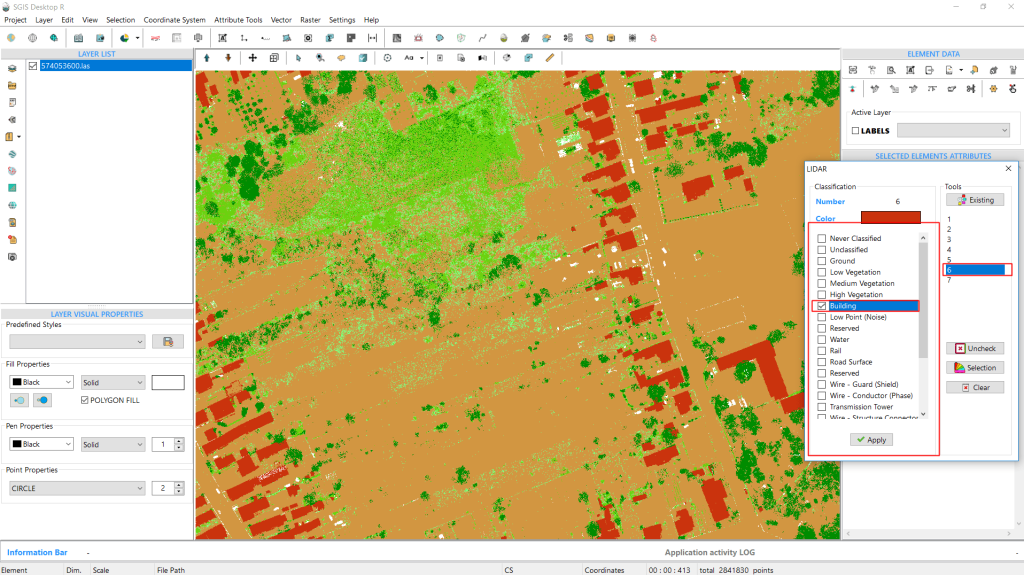
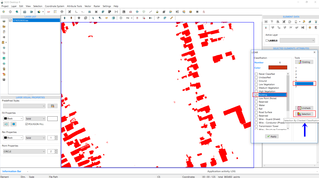
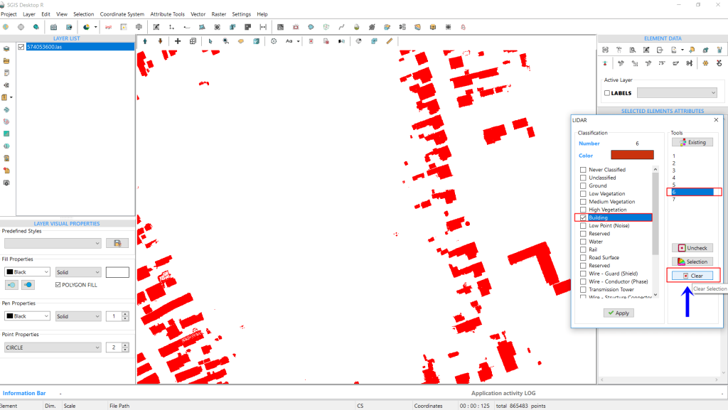
After importing a LAS file, click on the ‘LIDAR’ function. In the Tools tab, select ‘Get Existing Classifications.’ Once they are displayed in the memo box, click ‘Uncheck non-existing’ to simplify the list. Now, in the Classifications tab, uncheck all but the ‘Buildings’ class for demonstration purposes. Click ‘Apply’ to transfer these settings to the graphics panel, where only the Building classification will be visible. If you want to reset or choose a different classification, simply click ‘Clear’ to remove the current selection.
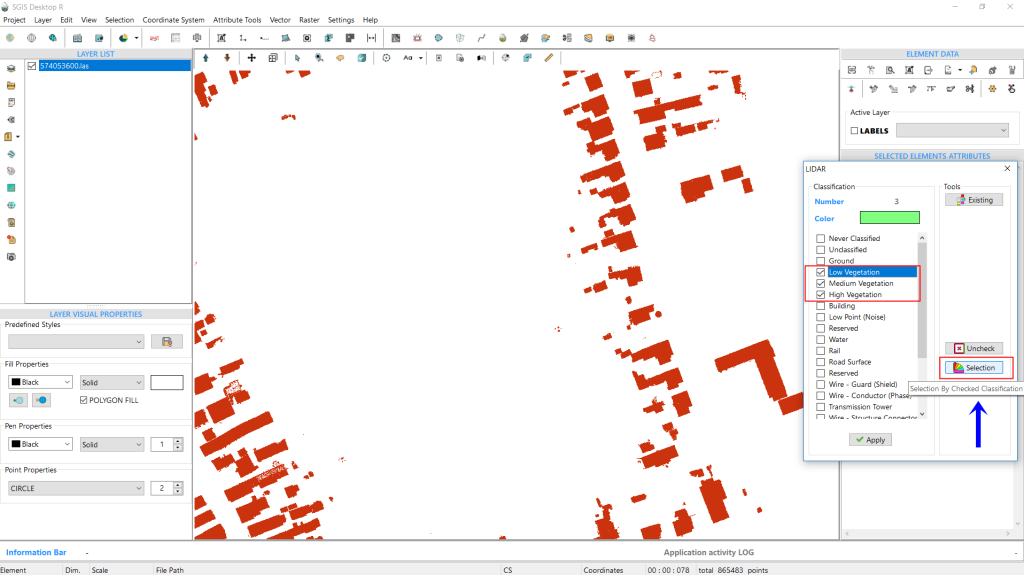
You can also select and highlight multiple classifications at once. For example, to select low, medium, and high vegetation classifications, simply check all three boxes and click on ‘Selection By Checked Classification’.
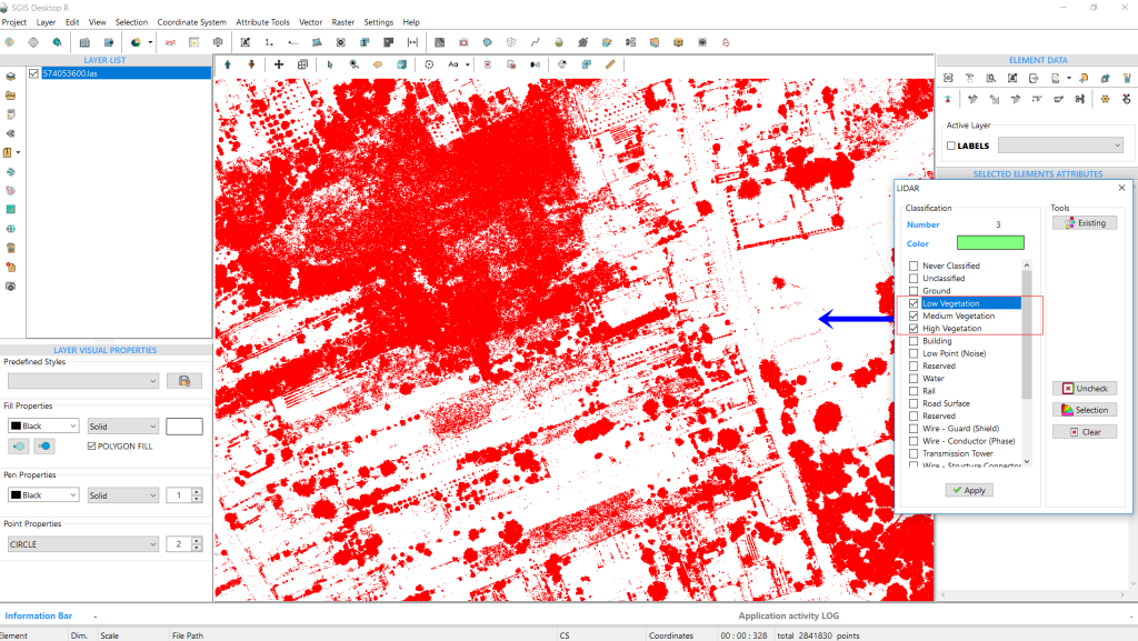
All vegetation classifications are instantly selected and highlighted in red within the graphics panel.
To isolate these points into a separate GIS layer, simply click on the ‘Selected in New Layer’ function.
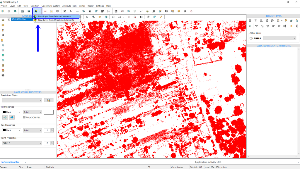
The function will prompt you to name the new layer. We’ll enter ‘Vegetation’ and then click ‘OK’ to proceed.
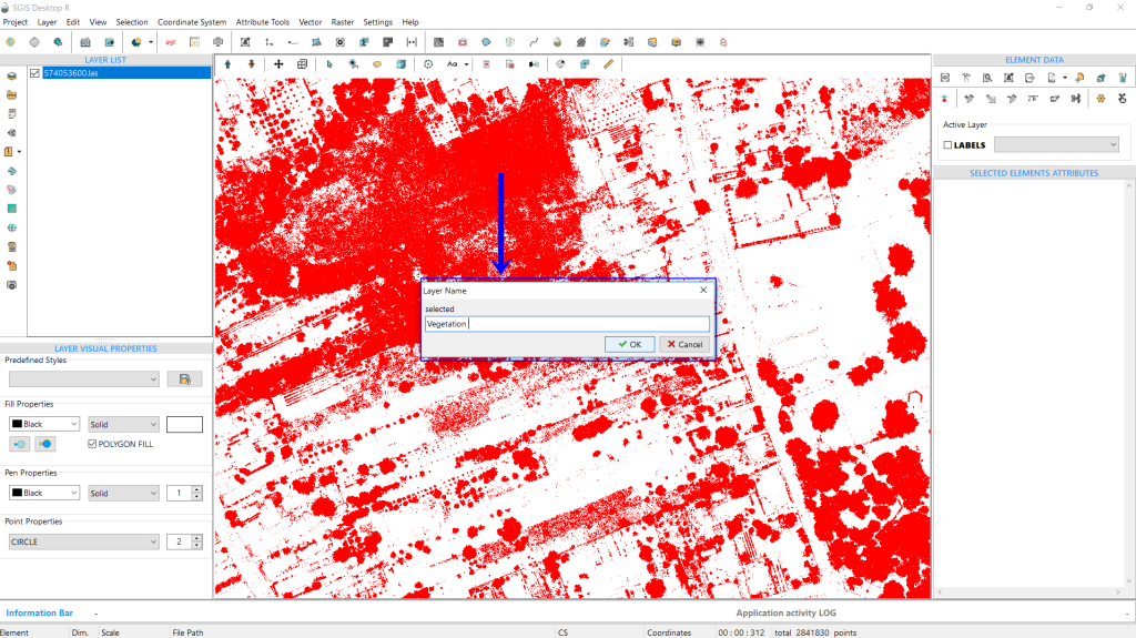
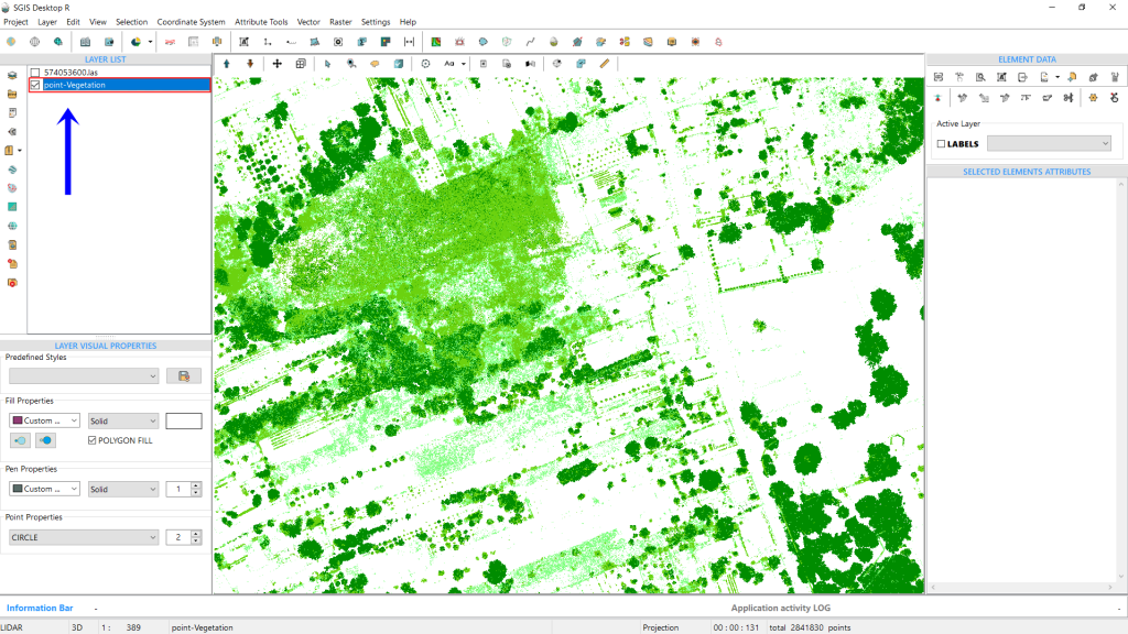
The new layer, containing only Low, Medium, and High Vegetation classifications, is immediately created and visible in the Layers panel.
This completes the procedure.
Inverse Distance Weighting (IDW) is a common spatial interpolation method used to create continuous surfaces, such as Digital Elevation Models (DEMs) or hillshades, from LiDAR point clouds. LiDAR data consists of discrete points, each with specific coordinates and elevation values, but to perform meaningful terrain analysis—like generating hillshades or contour maps—a continuous surface is needed.
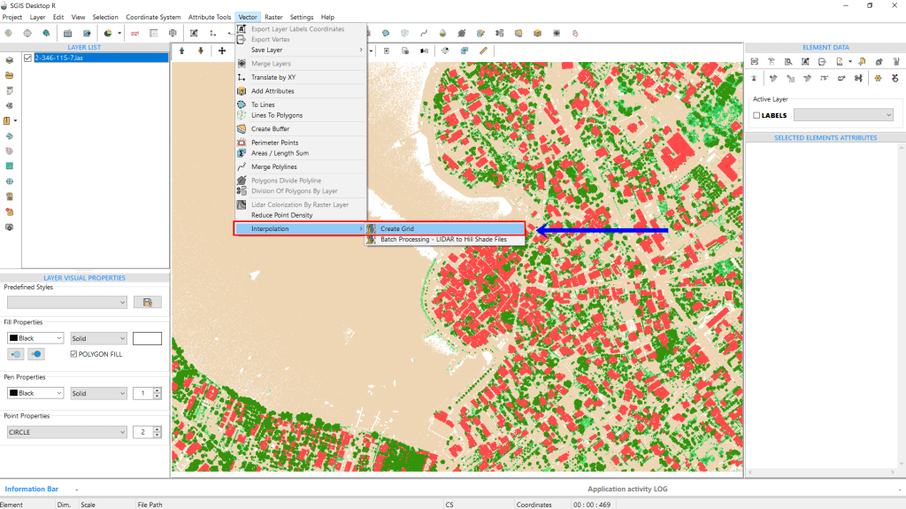
In SGIS v.R, this process is straightforward. To begin, we simply open the ‘Create Grid’ tool. Once selected, a new dialog window will appear.
We’ve already imported the LiDAR point cloud, so now we’ll focus on explaining the settings and options within the function.
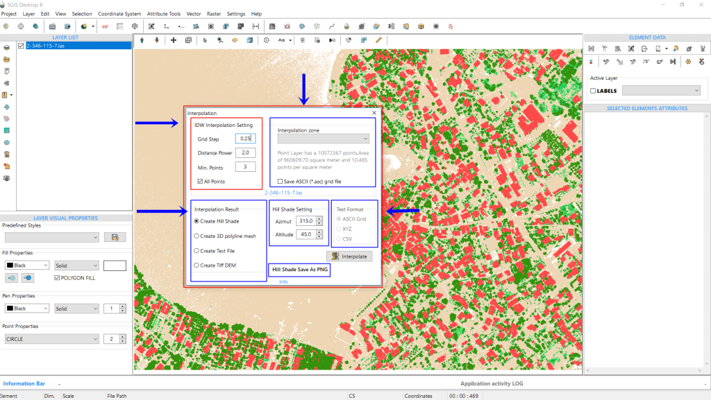
In the ‘Interpolation Settings’ box, we can see that the point cloud contains 10,072,367 points, covering an area of 960,609.70 m², with average density of 10.485 points per square meter. This provides a sense of the data’s size, showcasing the efficiency of the algorithm, which completes the process in under a minute.
Moving to the settings, the first box includes the IDW interpolation parameters.
Here, you’ll find an empty field for “Grid Step,” where users can input their preferred value (default is set to 1m).
The “Distance Power” is set to 2 by default, though this can be adjusted as needed.
The “Min. Points” option is set to 3 by default, and there’s also a checkbox labeled “All Points”.
For this example, we’ll set the “Grid Step” to 0.25m, while leaving the “Distance Power” and “Min. Points” at their default values of 2 and 3, respectively.
The next box in the settings is for defining the interpolation zone.
If your input point cloud doesn’t have a fixed extent—meaning the points form an irregular shape—you’ll need to add a polygon layer and select it as the interpolation zone.
The ‘All Points’ checkbox and the ‘Interpolation Zone’ setting are key options, and users must select one or the other.
If the area to be interpolated is rectangular, simply choose ‘All Points.’
However, for irregularly shaped areas, users need to add a Polygon layer (whether in Shapefile, GML, or GMT format) to the Layers Panel. Then, from the Interpolation Zone dropdown list, they can select the desired area (zone) for interpolation.
In this example, since we’re working with a fixed extent, we’ll leave this field empty. Below, there’s a checkbox labeled “Save ASCII” that allows users to automatically export an ASCII file (ASC Grid format file) from the process into the same folder.
We’ll leave this unchecked as well.
At the bottom of the interpolation dialog, you can adjust the output settings. The first box lets users choose the type of output they want. You need to select one option before running the procedure.
The options include generating a hillshade, creating a 3D polyline mesh, saving the output as a text file, or producing a Tiff DEM.
On the right side, you can adjust the azimuth and altitude values for the hillshade—default values are 315 for azimuth and 45 degrees for altitude.
In this example, we’ve checked the first box to display the hillshade directly in the Layers Panel. If a user chooses to save the output as a text file, the third settings box will activate, offering format choices like ASCII grid, XYZ, or CSV.
Additionally, the hillshade can be exported as JPG, TIFF, or PNG.
Once all desired settings are configured, we click “Interpolate” to run the procedure.
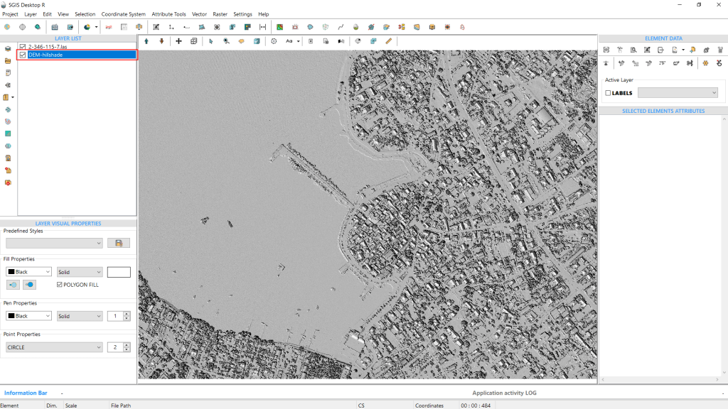
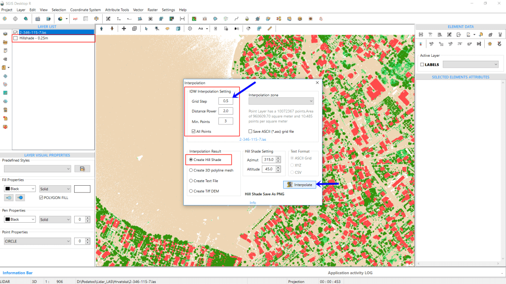
We’ll run the process two more times to create hillshades with grid steps of 0.5m and 1m.
Afterward, we’ll compare the results of all three.
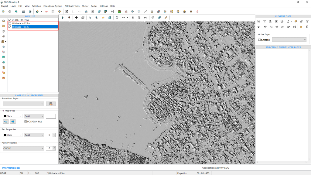
The process is repeated a third time, producing a hillshade with a grid step of 1m.
We will save all three hillshades as PNG files.
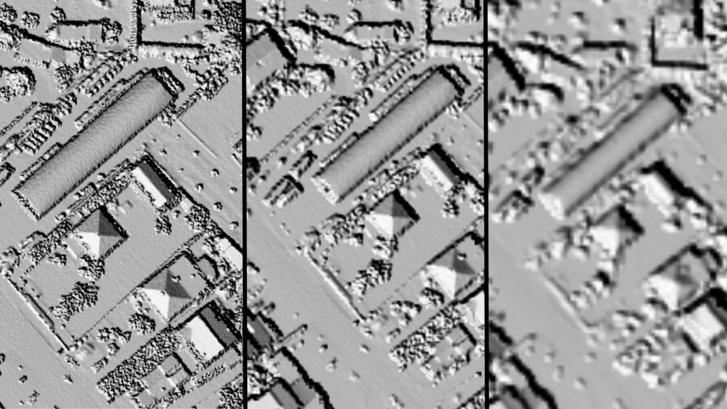
In Fig.32, the difference in raster quality is clear. The first image highlights the hillshade with a 0.25m grid step, followed by the 0.5m grid step in the second image, and finally, the 1m grid in the third.
It’s evident that the sharpest and highest quality DEM is produced with the 0.25m grid step.
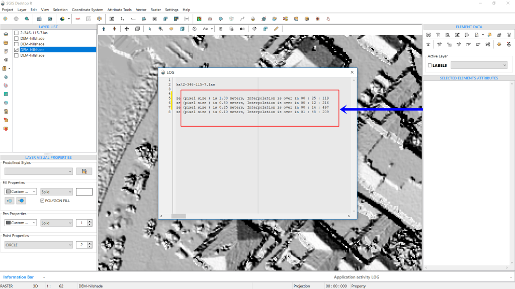
Another notable feature of SGIS v.R is its ability to export a LOG file detailing all procedural steps and their respective durations. For instance, the LOG file indicates that creating a Hillshade DEM with a 1m grid step took 25 seconds and 119 milliseconds. The time is recorded in the format of minutes:seconds:milliseconds (00:00:00).
For a grid step of 0.5m, processing the entire point cloud took 12 seconds and 216 milliseconds. Meanwhile, generating the Hillshade DEM with a 0.25m grid step took 14 seconds and 497 milliseconds.
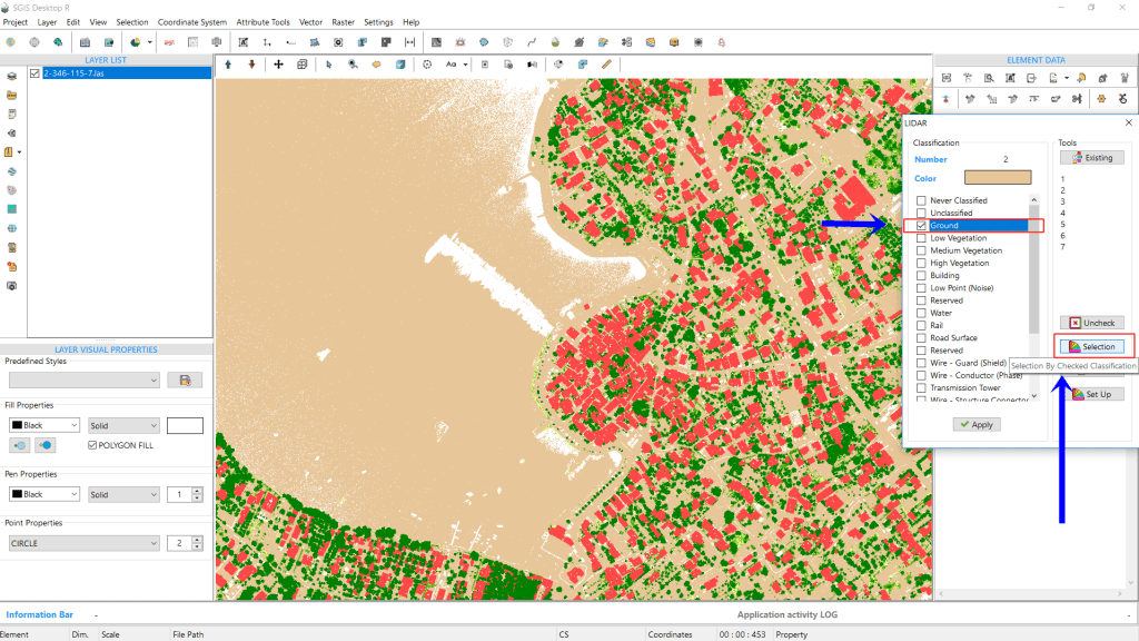
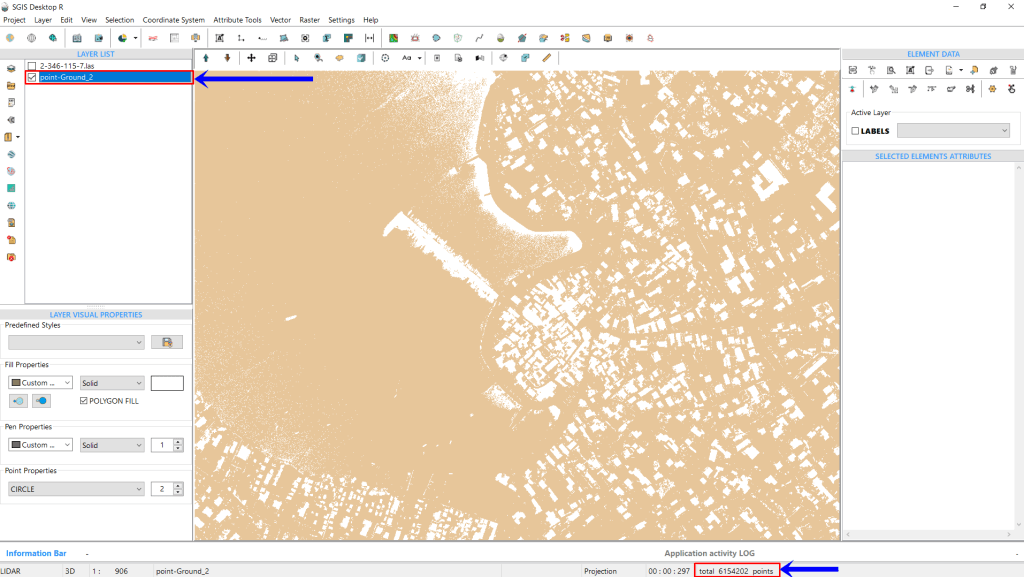
Next, we’ll use the same point cloud to generate a DTM hillshade. Since the LAS point cloud is already imported, we’ll go back to the ‘LIDAR’ toolbox. Here, we’ll ensure that only the ‘Ground’ classification is checked. Using the ‘Selection By Checked Classification’ function, we’ll isolate the ground points and create a new GIS layer in the Layers Panel.
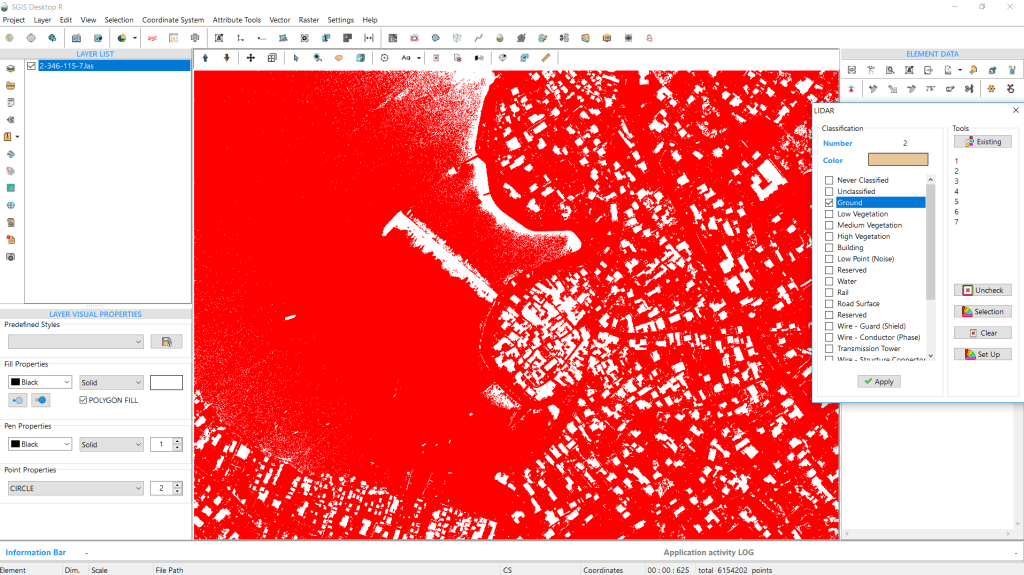
The information toolbar in the corner will display the number of points in this ground layer. Once that’s set, we’ll open the ‘Create Grid’ tool to adjust the settings.
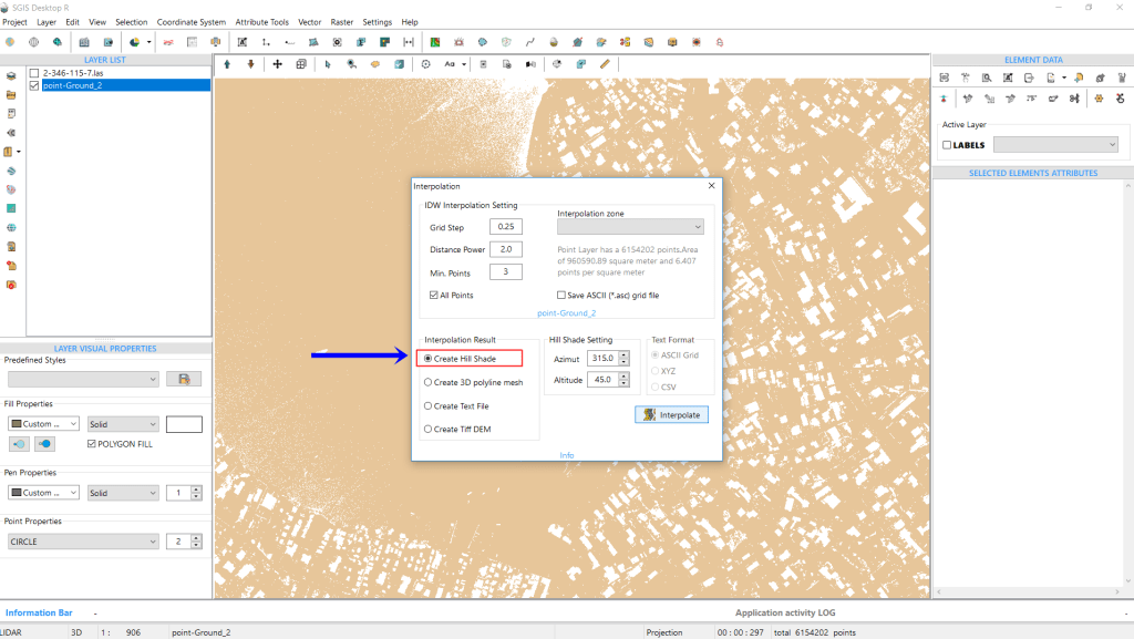
In the Interpolation dialog, we’ll adjust both the input and output settings. Since we’re generating a DTM hillshade, we’ll use the same settings as before. The Grid Step will be set to 0.25m, with the Distance Power at 2 and Min. Points at 3.
For the output, we’ll select ‘Create Hillshade,’ keeping the default Azimuth at 315 degrees and Altitude at 45 degrees. Once everything is set, we’ll click ‘Interpolate’ to generate the hillshade.
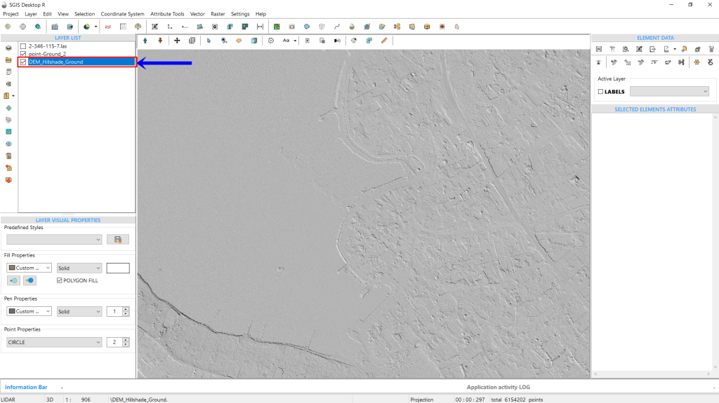
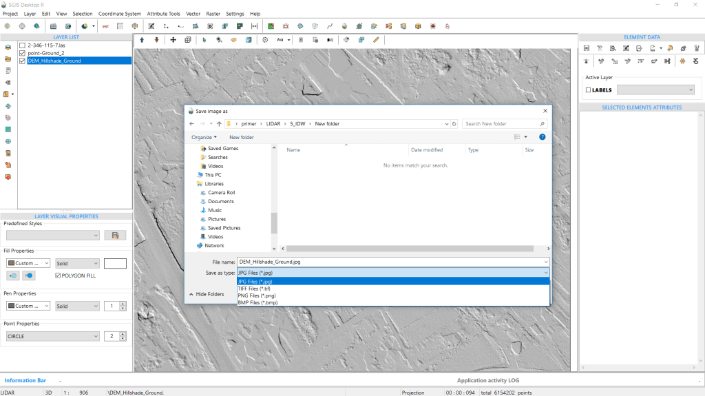
The hillshade can be exported as a raster file in several formats, including PNG, TIFF, JPG, or BMP. Along with the raster file, the software generates a corresponding world file to ensure the hillshade is georeferenced and properly aligned.
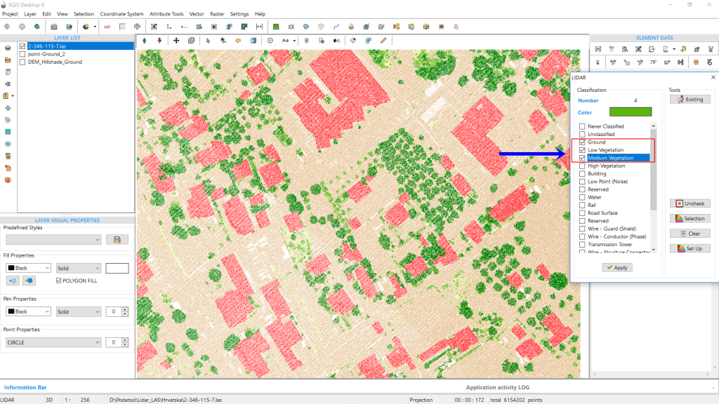
For demonstration purposes, we’ll export a DEM hillshade that includes multiple classifications, such as ground, low, and medium vegetation. This shows that the algorithm can handle combinations of different classifications, not just a single one. The process remains the same, but this time, we’ll keep three classes selected in the ‘LIDAR’ toolbox: 2, 3, and 4.
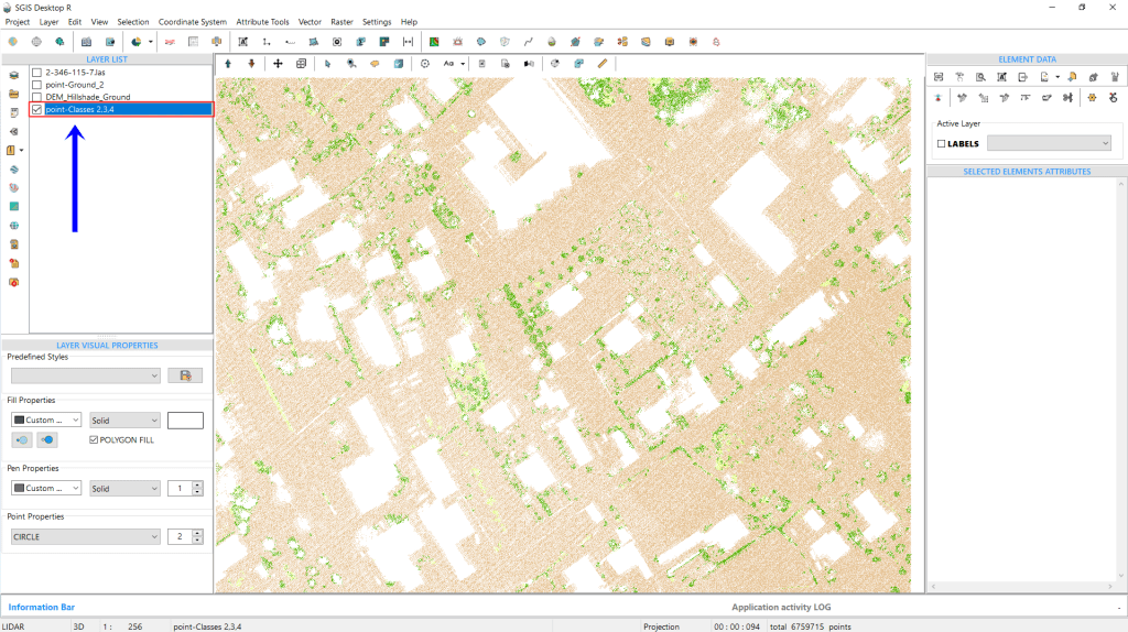
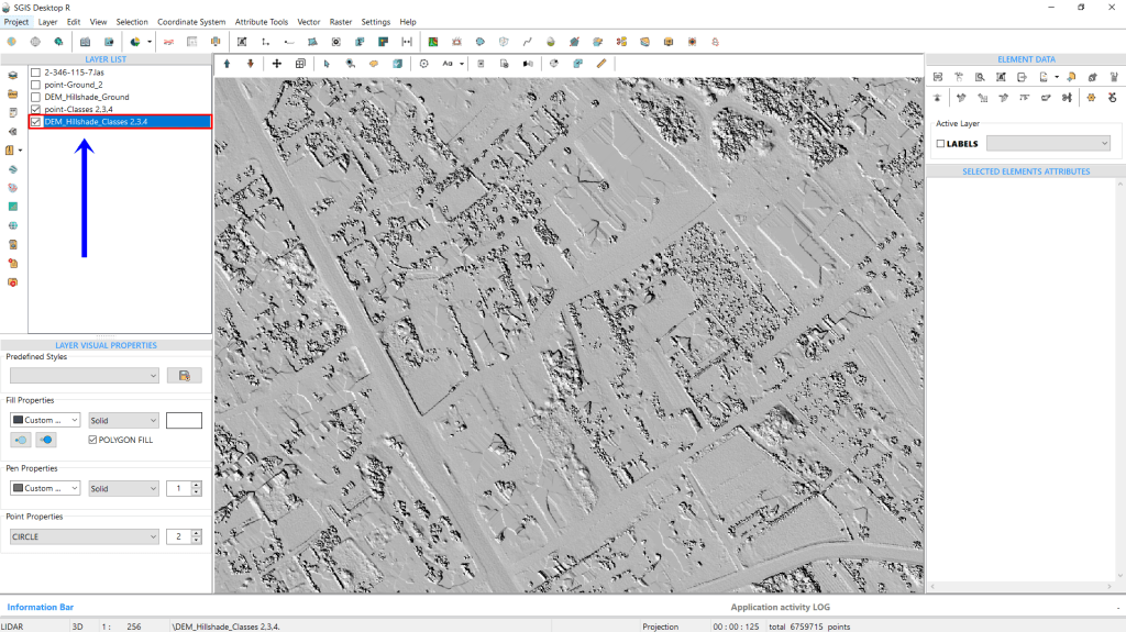
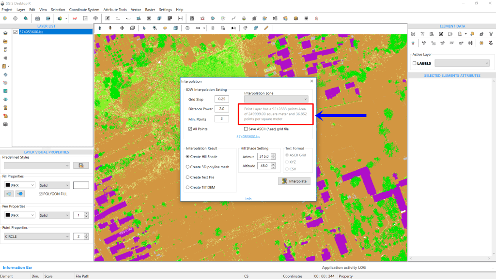
To conclude our analysis, we will add another LAS file, which contains 9,212,883 points covering an area of 249,999.99 m². The average point density is about 36.85 points per square meter, significantly higher than the previous LAS file, where the average was 10.5 points per square meter. With this denser dataset, we can interpolate using a Grid Step of either 0.1m or 0.25m. To determine which provides better results, we’ve exported hillshades for both grid steps.
The results are as follows:
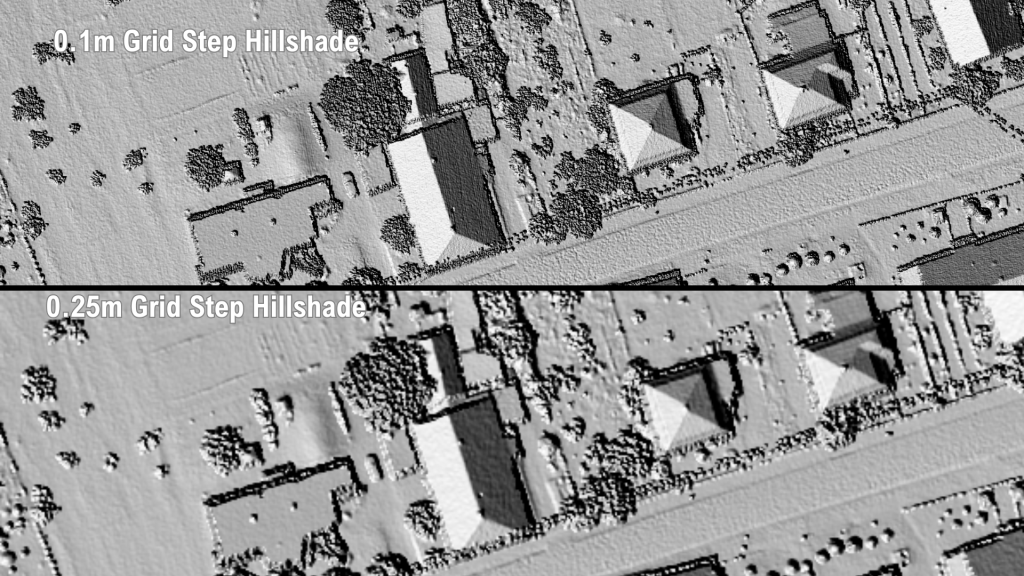
With an average point density of around 37 points per square meter, it’s clear that a 0.1m grid step delivers better results. This analysis highlights that a 0.25m grid step isn’t always optimal. The dataset itself determines the ideal grid step for the best output. For a dataset with an average point density of 10.5 points per square meter, the 0.25m grid step offers the best results. Similarly, when working with a denser point cloud—about 37 points per square meter—a 0.1m grid step yields the highest quality hillshade.
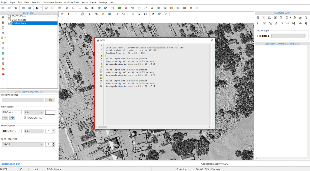
Additionally, the time taken for these processes is noteworthy. From the LOG file, we see that generating a hillshade with a 0.25m grid step took 10 seconds and 545 milliseconds, while the 0.1m grid step took 21 seconds and 714 milliseconds.
Batch processing LAS files to generate DEM hillshades is a valuable tool in GIS, especially when working with large datasets like LiDAR point clouds. By automating the processing of multiple files at once, it saves time and reduces the manual effort involved, which is particularly beneficial for large-scale projects. This method accelerates the creation of Digital Elevation Models (DEMs), offering a faster workflow compared to handling each file individually.
When working with large LiDAR datasets, batch processing makes it easier to manage the data efficiently. It also ensures that settings and outputs are consistent across all files, reducing the chance of human error and producing uniform results. Overall, automation not only speeds up the process but also allows users to focus more on analyzing the results, rather than performing repetitive tasks.
SGIS v.R provides this feature to automate the generation of DEMs or hillshades from multiple LAS point cloud files. This example demonstrates how to perform this task;
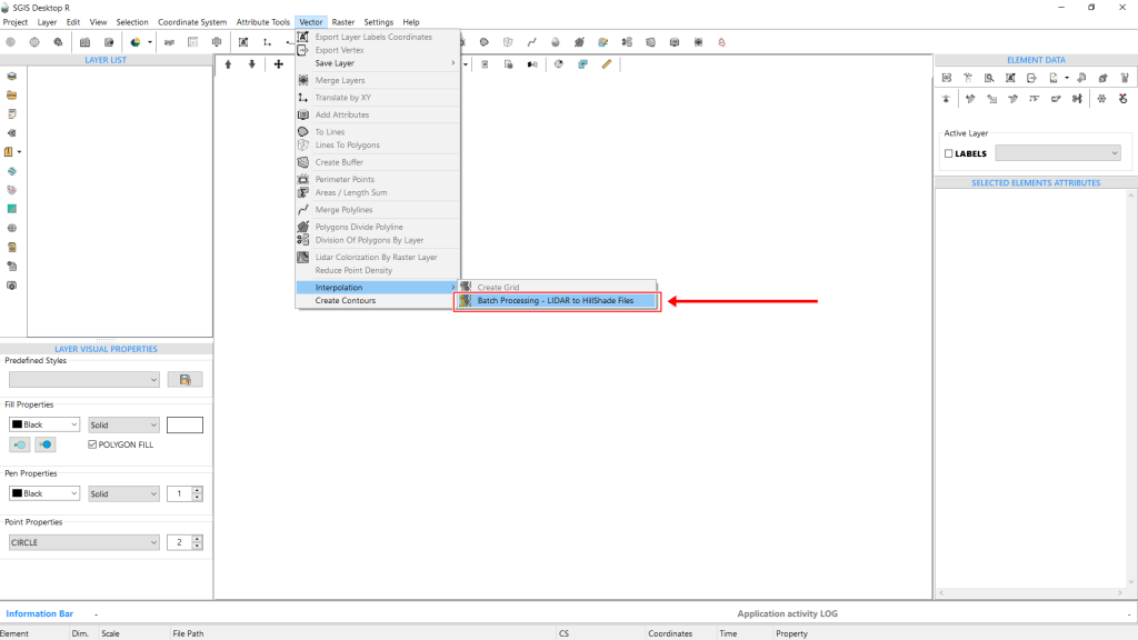
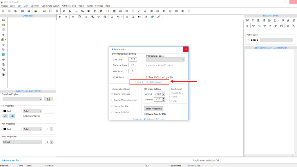
First, we need to open the ‘Batch Processing’ function from the main menu. Once selected, a settings dialog window will appear. Here, we can adjust the Interpolation Grid Step, which is set to 1m by default. For this example, we’ll change it to 0.25m. Next, we have the Distance Power, set at 2 by default, and the Min. Points, which defaults to 3. Users can modify these values, but we will leave them unchanged.
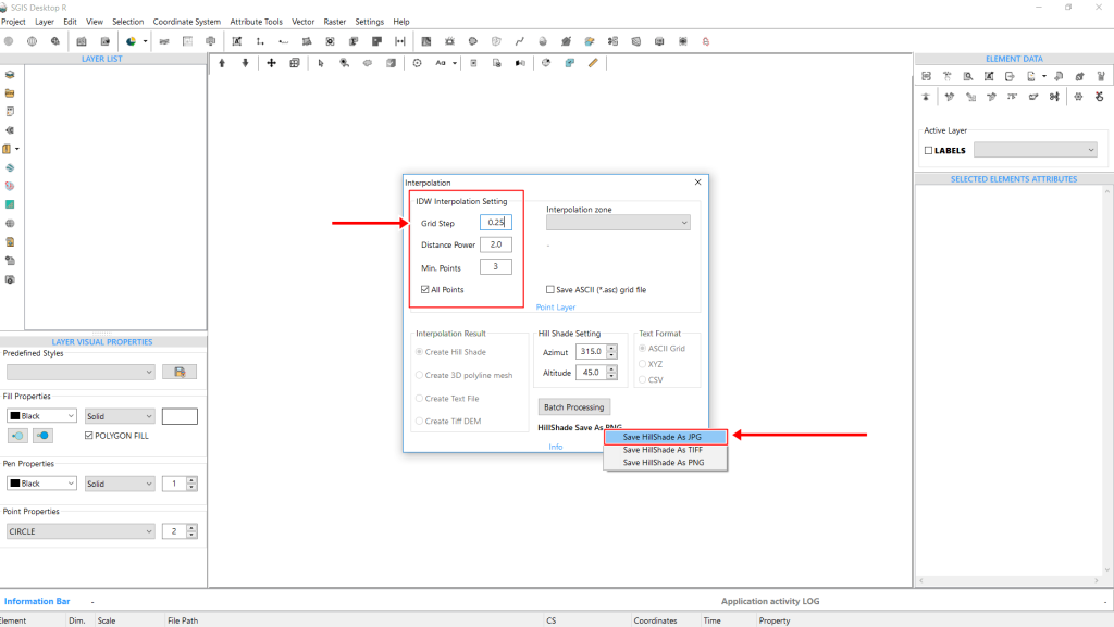
Next, the azimuth and altitude settings, they are set by default to 315 and 45 degrees respectively. We’ll keep these default values.
To save the hillshade, right-click and choose ‘Save Hillshade as.’ A dropdown menu will appear with options to save the files as PNG, JPG, or TIFF. For this example, we’ll choose JPG.
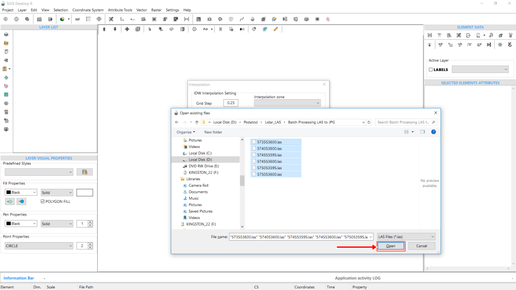
Next, click on ‘Batch Processing.’ This opens a file input window where the folder path needs to be selected, allowing us to choose all the LAS files from the folder.
In our case, we have six LAS files, and we will select all of them.
Now, simply click ‘Open’ to start the process.
A ‘Processing Toolbar’ in the dialog window will display the status of each file being processed and the number of files remaining.
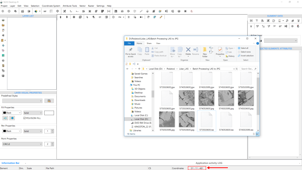
Once complete, you can open the folder and verify that the procedure was successful, with the JPG files and their corresponding world files generated.
In the lower info bar, you’ll see how long the operation took. For six LAS files with a grid step of 0.25m, the hillshades were generated in 1 minute, 11 seconds, and 481 milliseconds.
The timer is displayed as minutes:seconds:milliseconds (00:00:00).
Reclassifying LiDAR Points by selecting a specified elevation range involves filtering and reorganizing LiDAR data based on their elevation values. This process allows users to select points within a defined elevation range or to exclude unwanted points, such as noise or outliers that don’t meet the desired criteria.
Once filtered, the selected points are reclassified into different ASPRS categories. For instance, points can be categorized into ranges that represent terrain features like water, ground, low vegetation, high vegetation, or other relevant terrain elements. This improves data accuracy and clarity for further analysis.
To begin this process in SGIS v.R, we’ve already loaded two LAS files. We’ll walk through the procedure step by step, starting with activating the Selection tool.
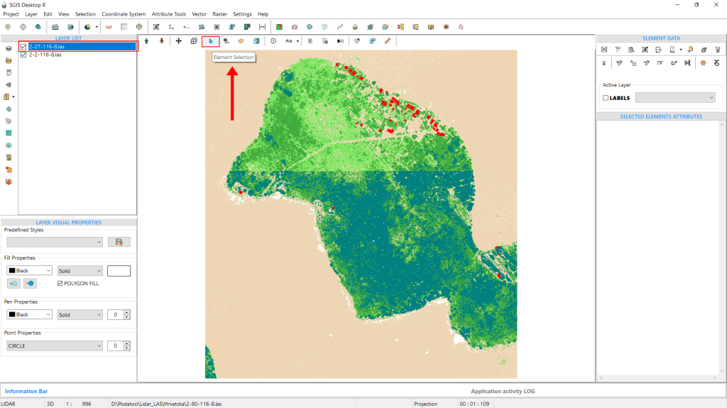
In our example, the LAS data depicts an island surrounded by water. Since the file is still undergoing quality control, the points representing water are currently classified as ground points.
To address this, we need to efficiently select all water points and reclassify them to class 9, which corresponds to water according to the ASPRS classification system.
We’ll use the ‘Selection By Elevation Range’ tool for this task.
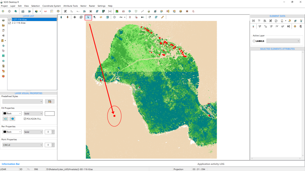
However, before proceeding, we first need to assess the elevation values in the area. To do this, we’ll activate the ‘Selection’ function. By simply clicking on the ground (which will later be reclassified as water), we can begin the process.
Without zooming in, we can select multiple points at once with a single click from the zoomed-out view. The software will then highlight the selected points in red.
The red highlighting is a customizable setting, which in this case, we’ve chosen as the default highlight color.
By pressing CTRL+S, the Layer Statistics dialog will open.
On the second tab, labeled “Details,” you’ll find the coordinates for the selected group of points, including the X, Y, and Z values.
If you scroll to the bottom of the list, you’ll also see the minH and maxH values, which represent the minimum and maximum elevation values for the selected points.
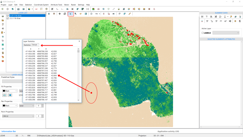
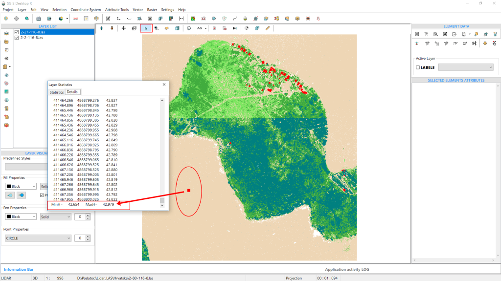
In this case, we can see that the minH is 42.654m, and the maxH is 42.979m.
Next, we’ll navigate to the Selection menu in the main ribbon and choose the ‘Select Elements By Elevation Range’ option. Then, we click on it to proceed.
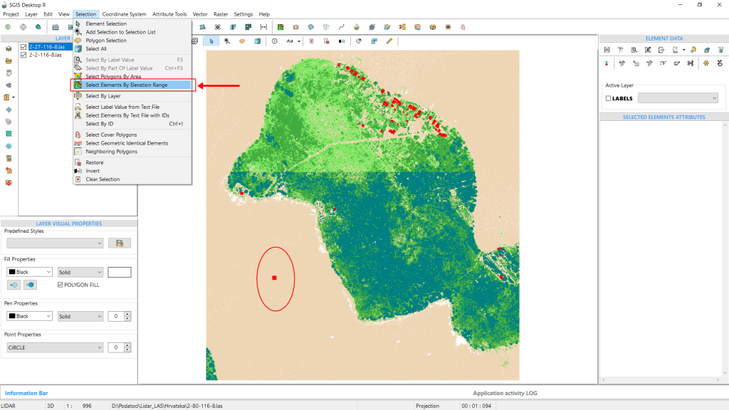
As soon as we click on the option, a dialog window appears, prompting users to select from three available options:
- We can check the first box to select points with an ‘Elevation less than…’ a specified value,
- The second box for ‘Elevation greater than…’ a given value, or
- The third option, ‘Elevation Between…’ for a range of values.
Since we already have both a minimum and maximum value, we’ll use these to input the elevation range.
Above the input fields, there’s a display bar that initially appears fully colored when the window opens, indicating that no filtering has been applied yet and all points from the active LAS layer are included.
After inputting our values from the example and pressing Enter, we immediately see the display bar adjust, showing that only a smaller subset of points falls within the selected elevation range.
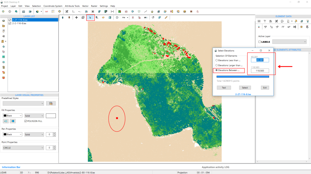
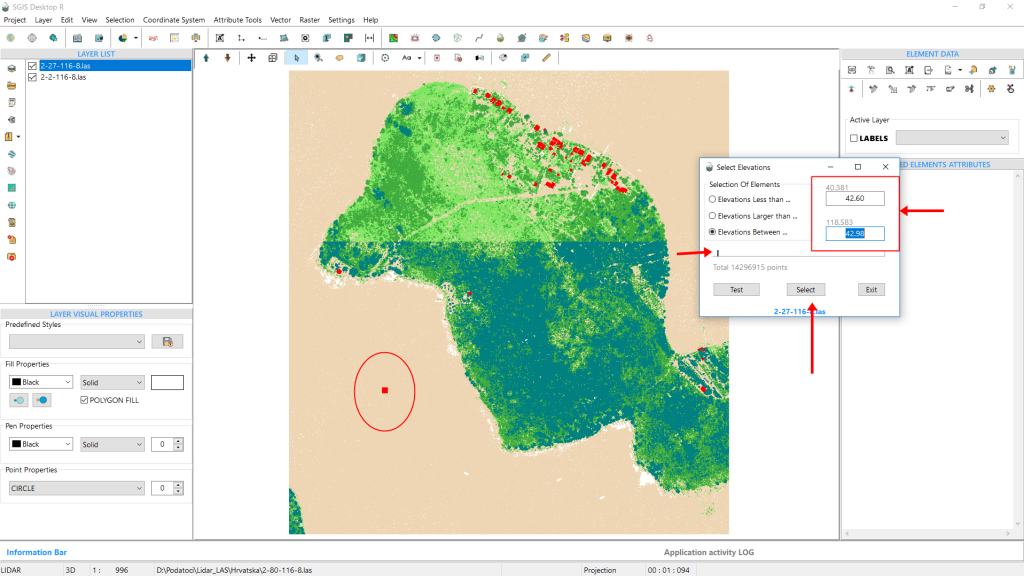
Next, we click on ‘Select.’ Once done, all points within the specified elevation range will be highlighted in the Graphics panel. We can now see that the ground points, which should be reclassified as water, have been accurately selected.
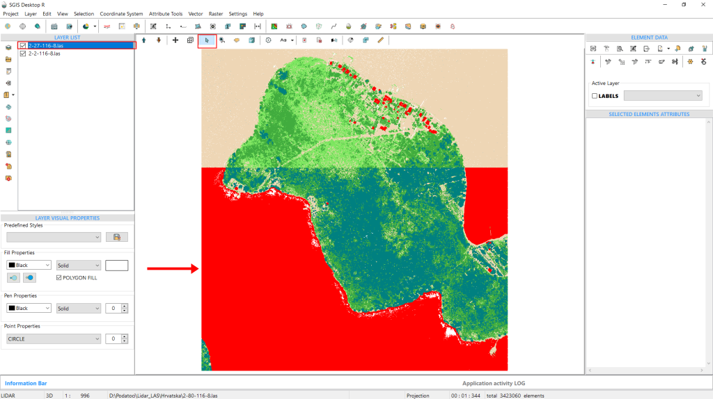
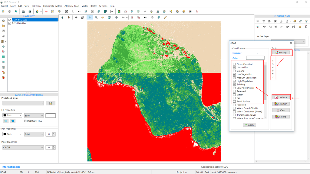
Next, we open the ‘LIDAR’ toolbox.
The selected points will stay highlighted unless we click ‘Clear Selection.’ First, we click on ‘Existing’ to display the current classification codes in the memo box, showing classes 1-7. To make things clearer, we click ‘Uncheck’ to deselect any empty classifications. Once it’s organized, we find and check the box for the Water classification. At this point, we can also choose a specific color to represent the water points.
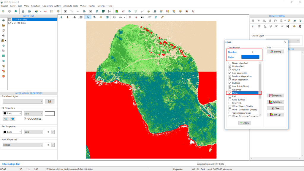
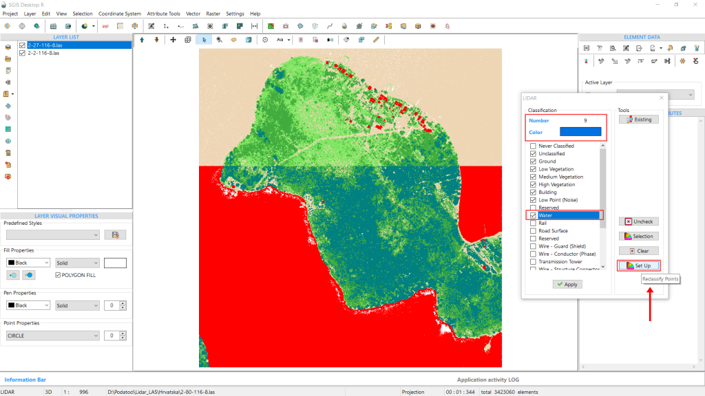
Once the settings are finalized, we click ‘Set Up’ to reclassify the points. All selected points are instantly reclassified into classification number 9, adopting the assigned color for that class.
The changes are reflected immediately in the graphics panel.
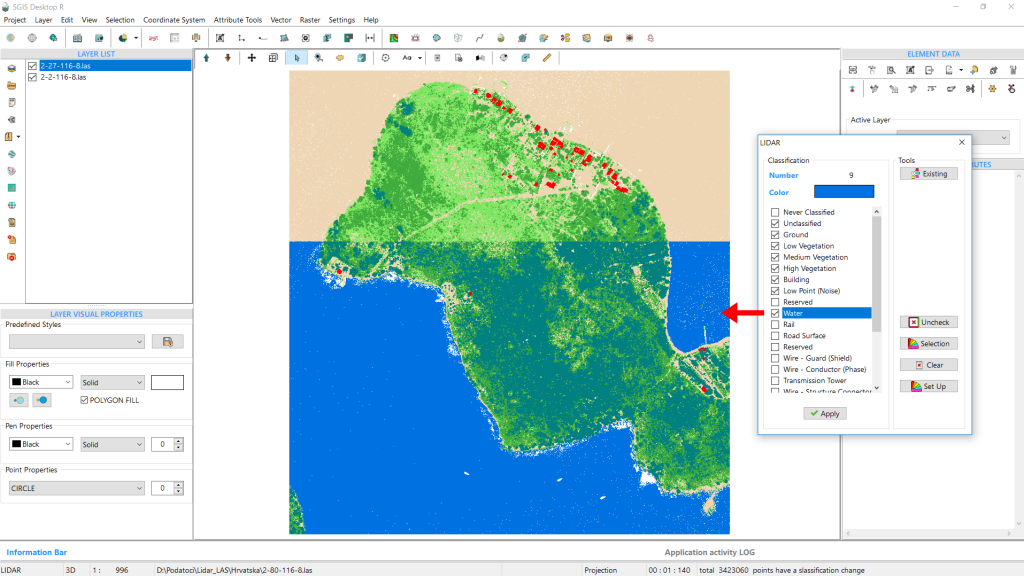
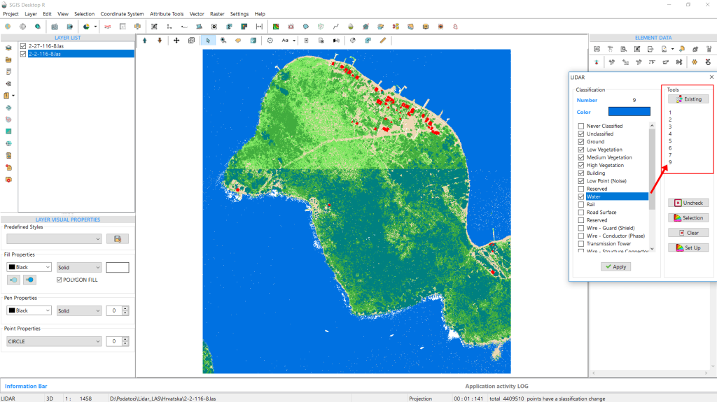
The previously ground-classified points have now been reclassified as water. Since this process was applied only to the first LAS file, we’ll repeat the same steps for the second file. Once the procedure is complete, and the water points are reclassified in both LAS files, we can select either file and, within the ‘LIDAR’ toolbox, click on ‘Existing’. At this point, classifications 1-7, along with class 9 (representing water), will appear in the memo list box.
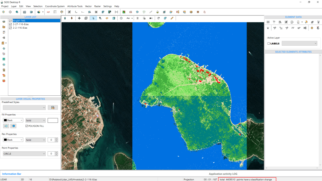
To wrap up, we can add a Tile basemap to enhance visualization and clarity. This completes the procedure.
Sometimes, we need to focus on a specific area of a LiDAR point cloud to create a raster, like a DEM or DTM. By narrowing down to just a portion of the data, you can save processing time and ease the load on your computer’s resources.
Let’s dive into how this is done in SGIS v.R.
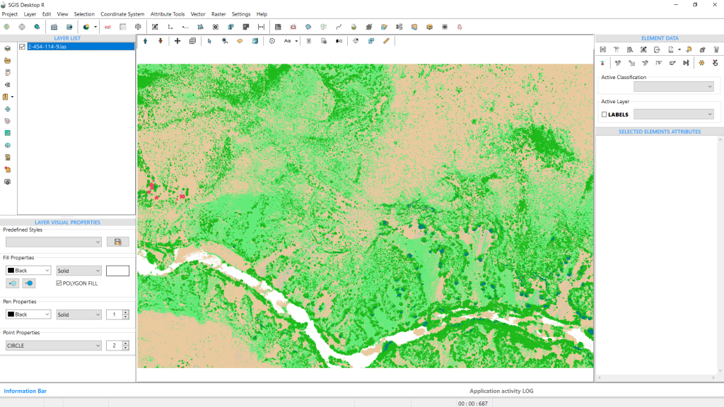
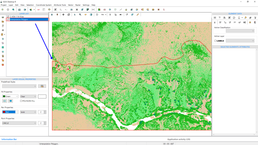
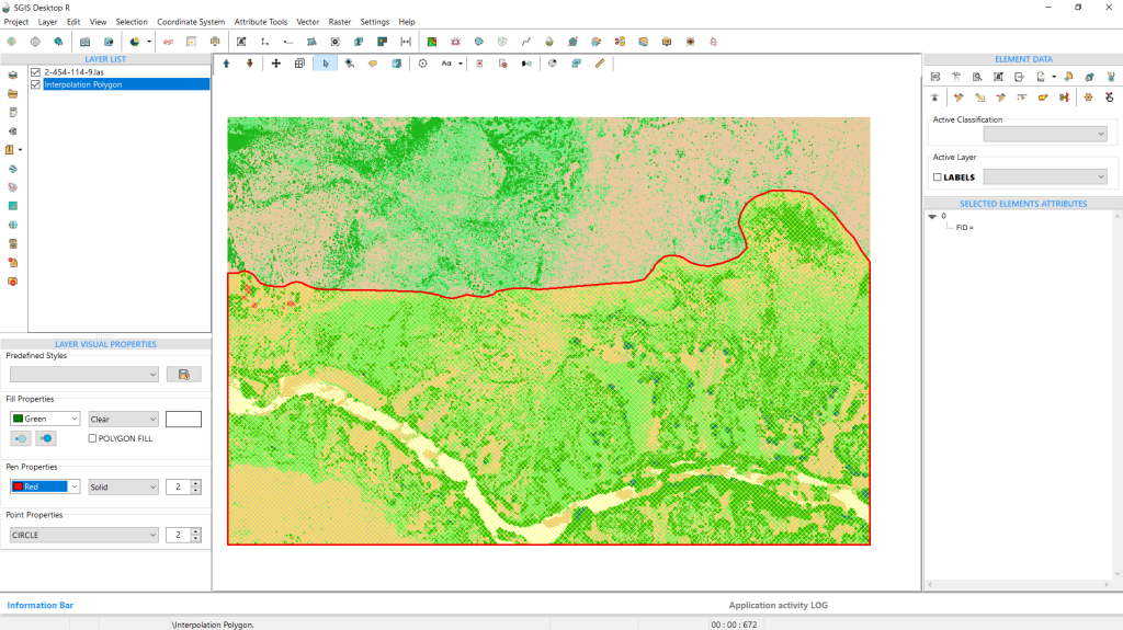
Once the LAS data is loaded, we’ll bring in the Polygon SHP layer. This polygon outlines the specific area we want to interpolate to a raster in our example.
Next, we need to find ‘Create Grid’ and click on it.
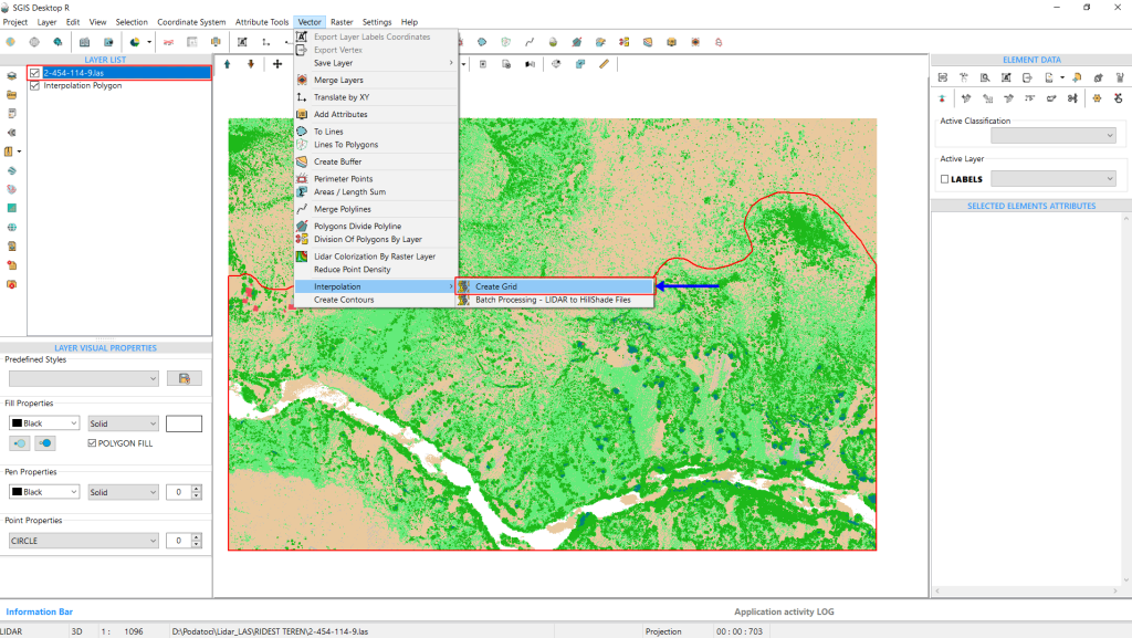
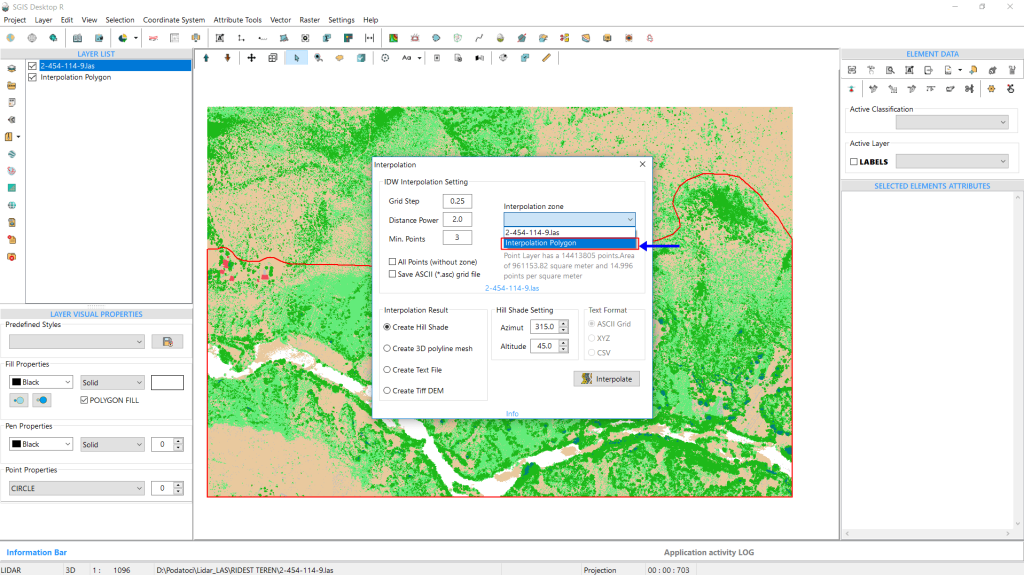
In the Interpolation dialog window, we need to adjust a few settings. First, we’ll set the Interpolation Grid Step to 0.25m, the Distance Power to 2, and Min. Points to 3.
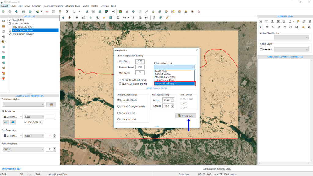
Instead of selecting ‘All Points’ like in the previous example, we’ll now choose the layer with the Polygon Area from the dropdown menu and click on it. The rest of the settings will stay the same. Finally, we’ll click ‘Interpolate’ to proceed.
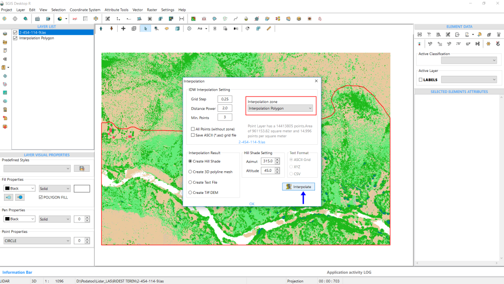
The DEM Hillshade is generated and displayed in the Layers Panel.
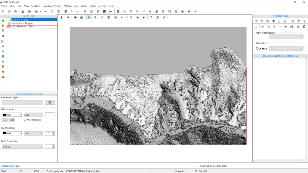
This Hillshade can be easily exported as a TIFF, PNG, or JPG file.
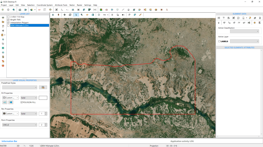
To highlight the area, we’ve overlayed a basemap with the polygon area, allowing us to visualize its location and the surrounding terrain features.
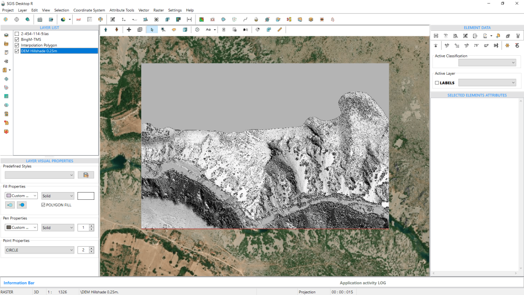
We’ll repeat the process, this time using the Ground Classification points to create a DTM for the selected area.
First, we’ll export the Ground points into a new layer in the Layers panel. To do this, we select Classification code 2 from the LIDAR toolbox, then close the toolbox and activate the ‘Selected Elements in New Layer’ function.
Once the Ground points are separated, we’ll open the Interpolation dialog window again and adjust the settings as needed.
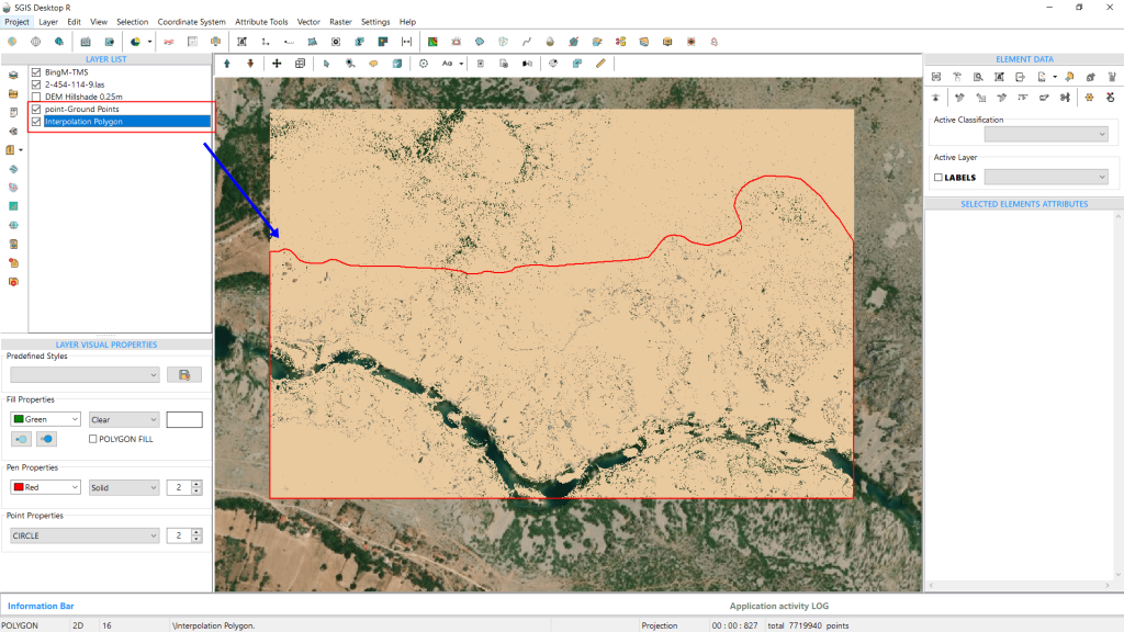
In the same way, we’ll set the grid step to 0.25m, the distance power to 2, and the Min. Points to 3. Since we’re using the same Interpolation Polygon area, we’ll select the ‘Interpolation Polygon’ layer from the dropdown list. With more layers now in the Layers Panel, these are reflected in the dropdown options. Once everything is set, we’ll click ‘Interpolate’ to proceed.
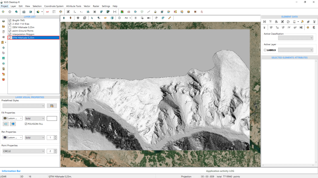
The DTM hillshade is generated in 859 milliseconds, as shown in the information bar at the bottom of the user interface. It can be exported as a raster file in TIFF, JPG, or PNG format for further processing. With that, the procedure is complete.
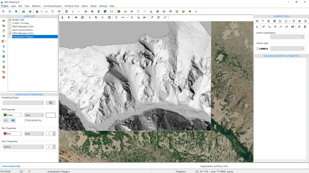
Handling large-scale LIDAR datasets, like multiple LAS files, can be a challenge. By defining project boundaries, users can focus on loading only the relevant data, making the process more efficient and cutting down on unnecessary processing. This approach prevents systems from becoming overwhelmed when dealing with large datasets, as it minimizes memory usage and computational strain. By working with smaller, more targeted sections of data, users can avoid slowdowns and boost processing speed, ensuring a smoother workflow overall.
SGIS v.R offers this feature through its ‘View LiDAR Boundaries’ tool. With this tool, users can easily select the number of LIDAR files they need, and it will automatically display the boundaries of all the selected files on the graphics panel. From there, users can quickly open any LAS file within the desired boundary for further analysis, making it a highly efficient way to manage and visualize large LIDAR datasets.
To illustrate how this function works, we’ll walk through a practical example by loading several LAS files into the software. This will give users a clear idea of how the tool operates and how easily multiple files can be opened and managed within the project.
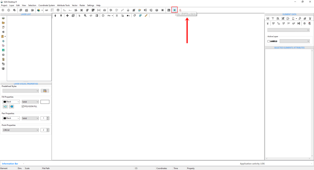
To get started, simply click on the tool.
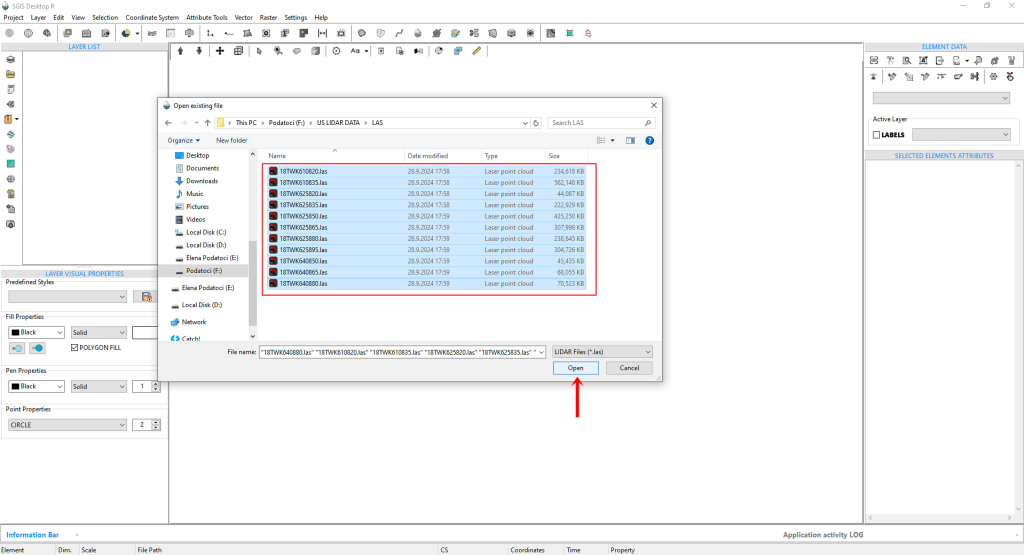
This will bring up an ‘Open File’ dialog box where you’ll need to navigate to the folder containing your LAS files. Once you’ve located the folder, you can easily select all the LAS files by clicking on one and then pressing CTRL+A.
All the files should now be highlighted and ready for the next steps.
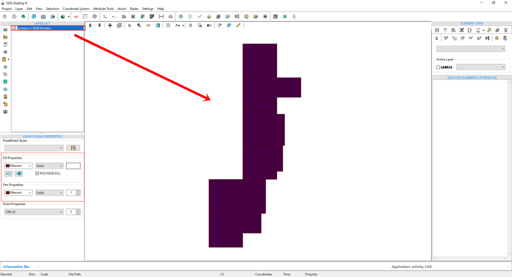
After clicking ‘Open,’ the LIDAR boundary polygons will quickly appear on the Graphics panel. Initially, these polygons will be filled with a random color. However, users have the option to customize the appearance by adjusting the pen and fill colors to their preference.
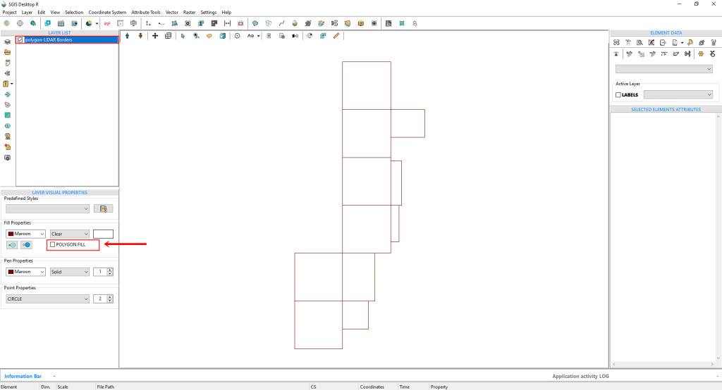
We’ll uncheck the ‘Polygon FILL’ option to remove the fill color inside the polygon areas. This adjustment will make it easier to work with as we import the LIDAR point cloud within these boundaries.
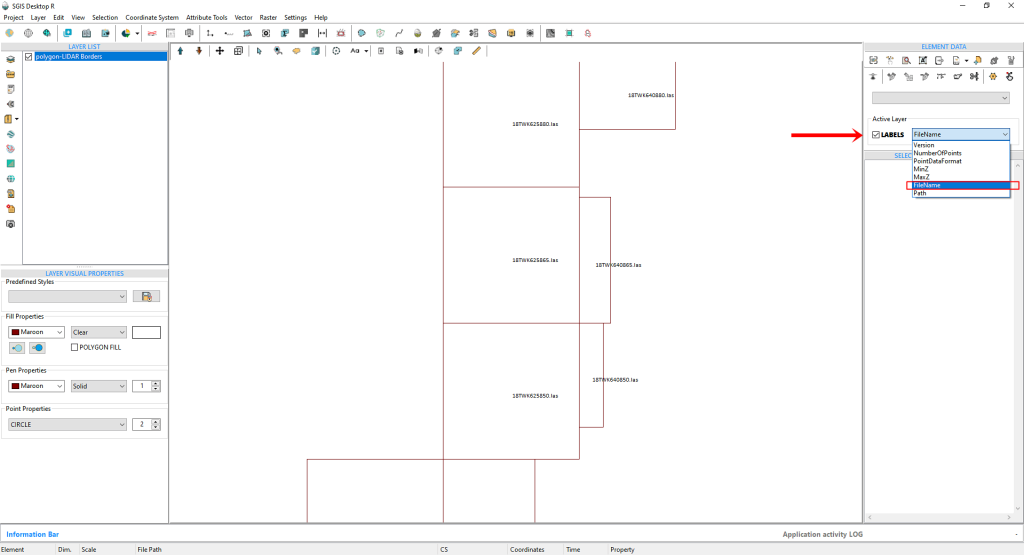
To streamline our workflow, we’ll activate the labels and choose the ‘FileName’ field from the dropdown menu. This will display the file name on top of each polygon, providing a clearer visual reference for users.
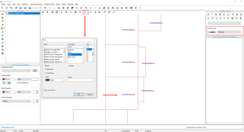
The Labels Visual Style can also be customized. By clicking on the ‘Font’ option, you can change the font type, style, size, height, color, and more. However, for the purposes of this demonstration, we’ll keep the current settings as they are.
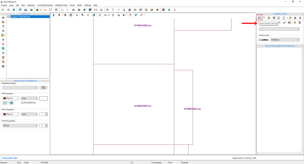
SGIS v.R offers an additional feature for managing labels on the Graphics panel called the ‘Label Visibility Border.’ This simple one-click option allows users to define a specific zoom level at which labels will be visible. When we activate this function, as shown in Fig.85, labels will appear when zoomed in and disappear when zoomed out. This helps prevent data overload on the graphics panel.
Let’s go ahead and click to activate this option.
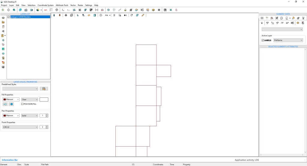
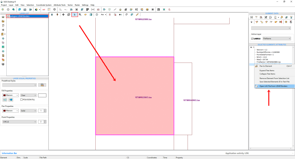
The next step in our process is to zoom in and select a specific polygon area. To do this, we simply need to activate the ‘Select’ function. By clicking on the polygon boundary, it will become highlighted, and in the ‘Selected Elements’ panel on the right side of the user interface, we can view the attributes of the selected polygon. We then click on any field displayed in the rows of the ‘Selected Elements’ panel and right-click on it. A dropdown menu will appear, where we can select ‘Open LAS file from Boundary’.
The LAS file has successfully loaded. Since it comes with predefined ASPRS classification color properties, we’ll open the LIDAR toolbox to adjust some of these settings for better visual clarity.
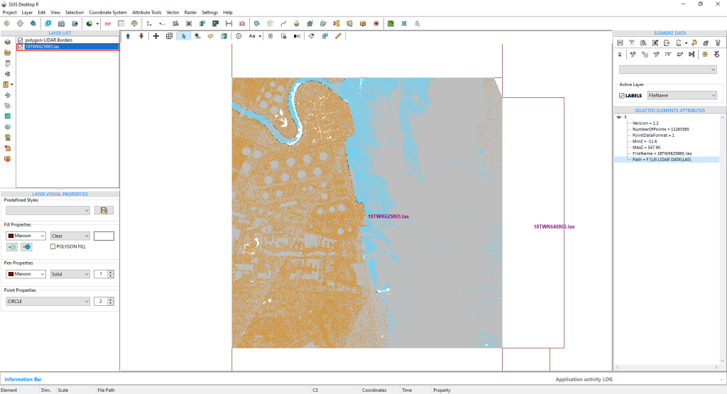
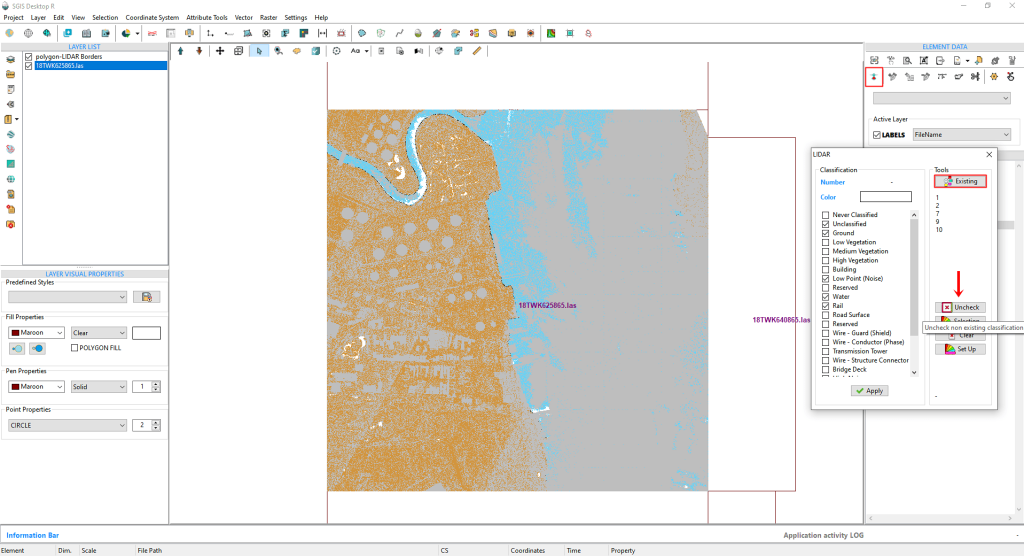
In the LiDAR toolbox, we start by clicking on ‘Existing’ to view the memo list of current classifications. Next, we select ‘Uncheck’ to deselect all empty boxes from the Classification list. For clearer visualization, we’ll also uncheck Class 1, as almost all non-ground points in this LiDAR dataset are classified as Unclassified.
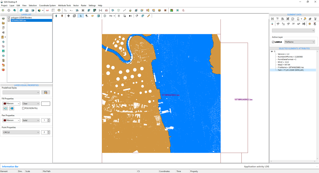
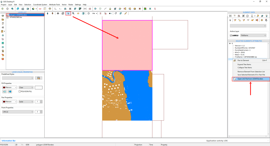
To open the second tile, we’ll activate the Selection function and simply click inside the next tile. After that, we can right-click on the ‘Selected Elements Attributes’ to open the second LAS file.
The LAS file loads instantly, retaining the visual settings we adjusted for the first file using the LiDAR toolbox.
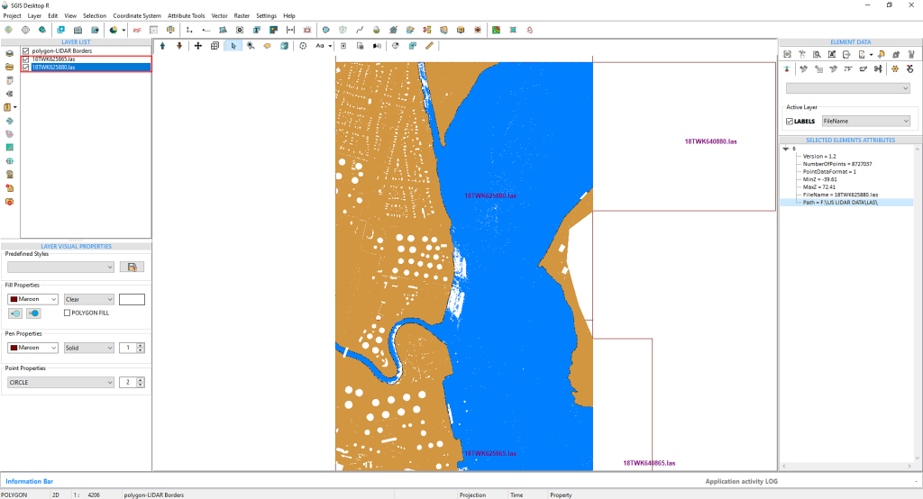
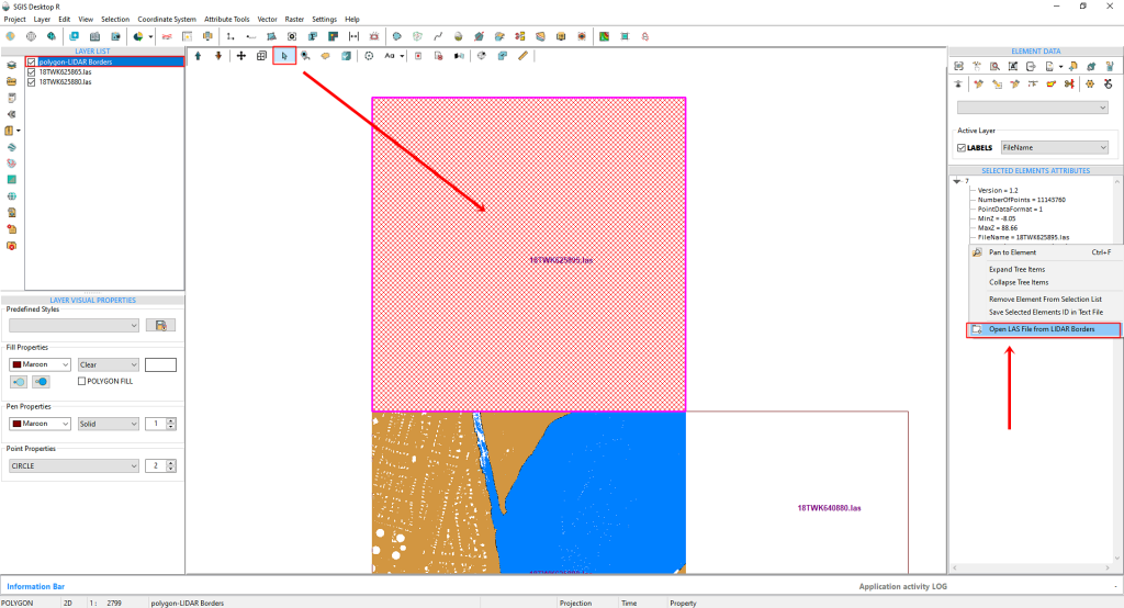
We’ll use the same approach to open the third tile, continuing this process for as many tiles as needed.
Additionally, we can load a Tile Map basemap to get a better view of the terrain and gain more insight into the urban area, as these LAS tiles are part of a city landscape. This extra layer helps in identifying features for further analysis or reclassification. To access the Tile Basemap, simply click on ‘Tile Map Servers’.
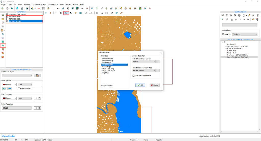
We’ll select ‘Google Satellite’ and then, on the right side, choose the ‘Coordinate System’ and ‘Transformation parameters’ from two dropdown menus. The coordinate systems are predefined with their EPSG codes, but users have the option to input custom settings and save them with an alias for easier recall.
For instance, we’ve already saved our coordinate system under the alias ‘USA18’ for quick reference and convenience.
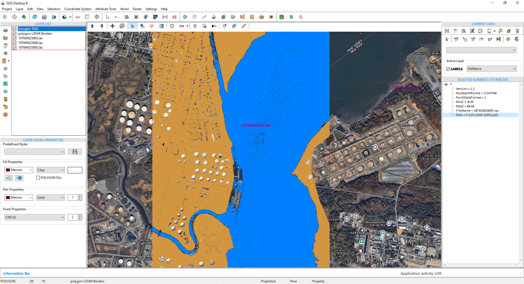
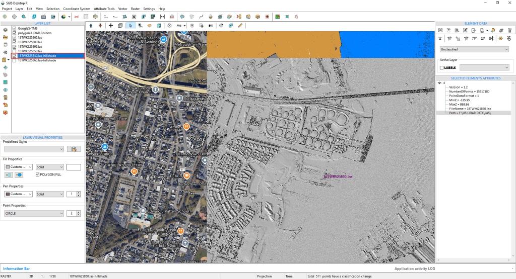
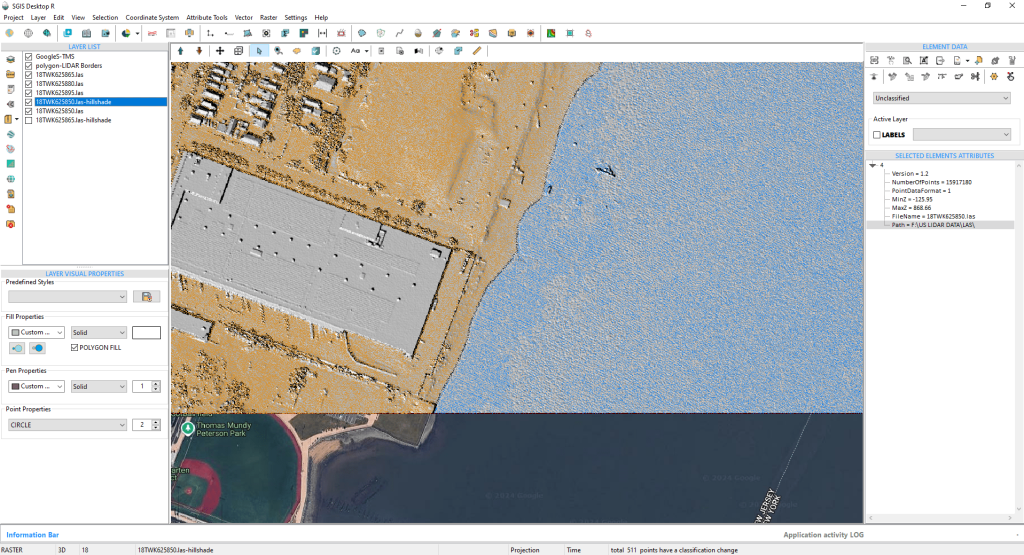
Users have the option to either add an existing hillshade layer or create one using the ‘Create Grid’ function. This enhances the three-dimensional visualization of the terrain, making it easier to detect elevation shifts, slopes, and subtle topographic features that may not be immediately apparent from the point cloud data. In urban environments like the one in our example, where natural and man-made structures coexist closely, a hillshade basemap helps users better visualize how features like buildings and roads interact with the surrounding landscape.
With this, the procedure is complete.
In GIS and related fields, ensuring the accuracy of LiDAR data is crucial for further analysis and processing. To achieve the best terrain representation, users often need to adjust their datasets to fit specific requirements or types of analysis. This might involve isolating building points or distinguishing vegetation (such as high vegetation) from other objects like buildings.
Manual reclassification becomes essential when automatic classification algorithms struggle to differentiate between similar features—like vegetation and low-lying structures. While automatic classification is a highly valuable tool, it can sometimes falter in complex or heterogeneous landscapes.
In these situations, the ability to manually reclassify points provides users with greater control over their data, allowing them to refine it as needed for better accuracy. This makes freehand LAS classification an indispensable feature for professionals who require high-quality, precise spatial data.
With SGIS v.R, users can easily draw freehand polygons on the graphics panel to select specific points. Once selected, the LiDAR toolbox can then be used to reclassify those points into a different category. Let’s walk through an example to see how this feature works.
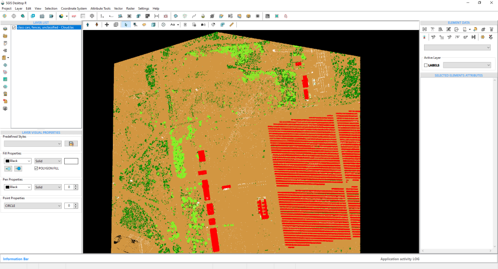
We’ve added a LAS point cloud, which contains classifications ranging from 1 to 7. For this example, we’ll focus on points representing a solar farm. Due to an error in the automatic classification, these solar farm points were mistakenly classified as building points. To correct this, we need to reclassify the building points from class 6 to class 1, which designates them as Unclassified points.
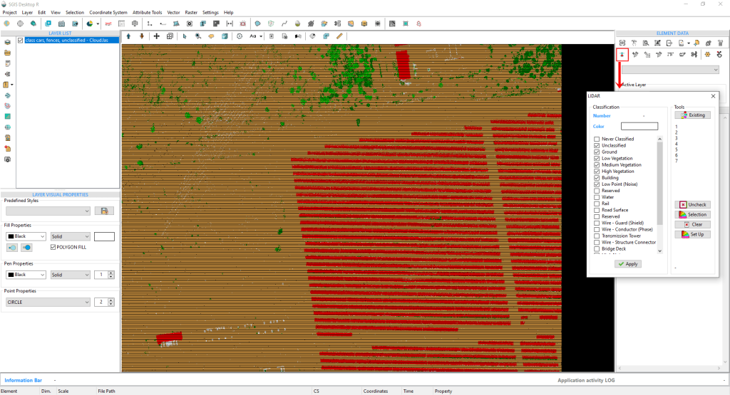
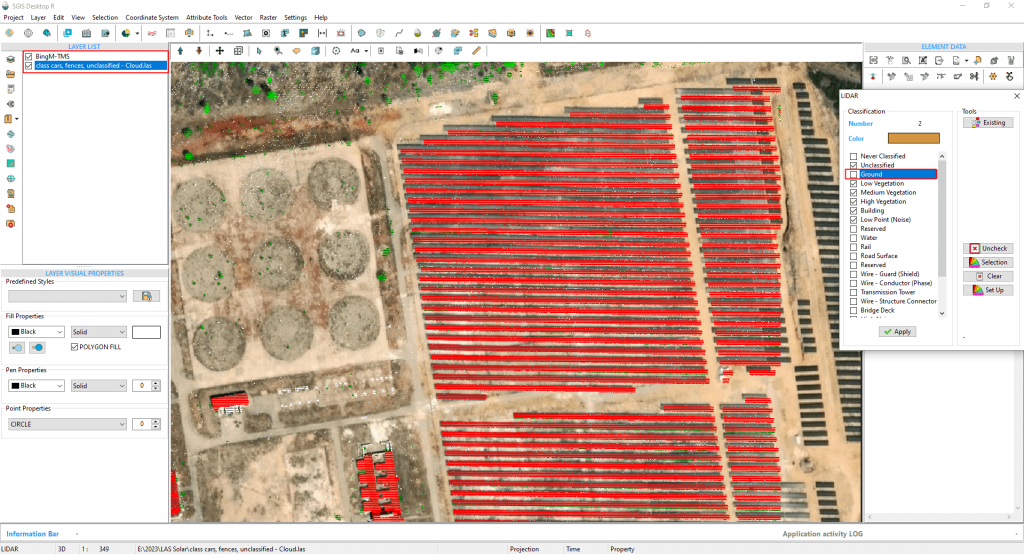
We’ve added a basemap to verify our observations. Now, let’s uncheck both the basemap and the ground points. We’ve also switched the background color from light to dark because a black background makes it easier to view and manage the points. Next, we need to check the point cloud layer and go to the Element Data panel to find the ‘Active Classification’ dropdown. From there, we’ll select ‘Buildings’.
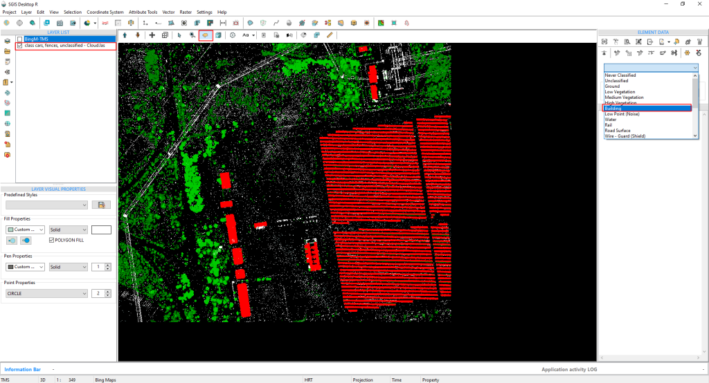
Next, we need to activate the ‘Polygon Selection’ function so we can draw a polygon on the Graphics panel. On the right side, the ‘Active Classification’ is set to ‘Building’.
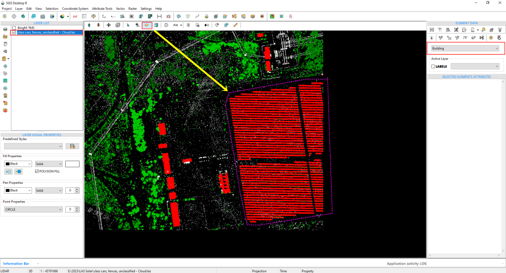
Once the polygon is drawn, the selected points will be instantly highlighted on the graphics panel.
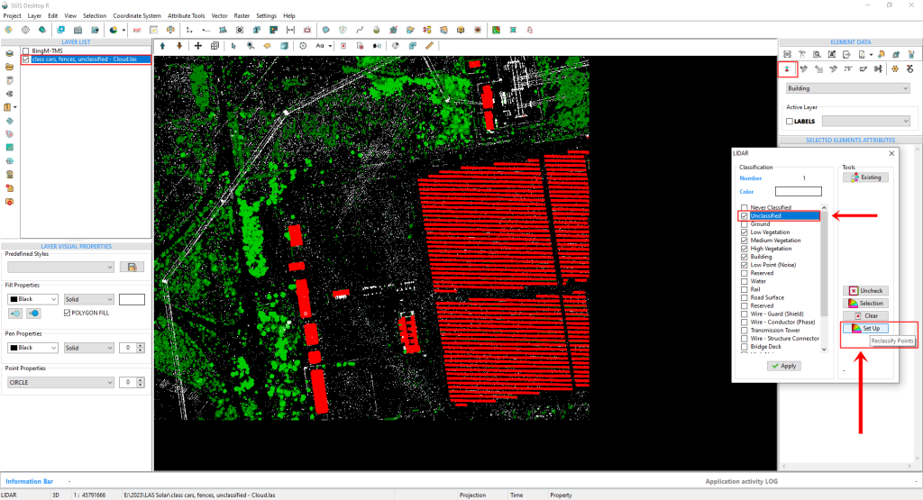
We will open the ‘LiDAR’ toolbox. In this section, we need to select the class where we want to move the chosen points. In our case, that’s class Unclassified or class 1. After that, we’ll click the ‘Set Up’ button. The points will be reclassified and moved to class 1, as shown in Figure 103.
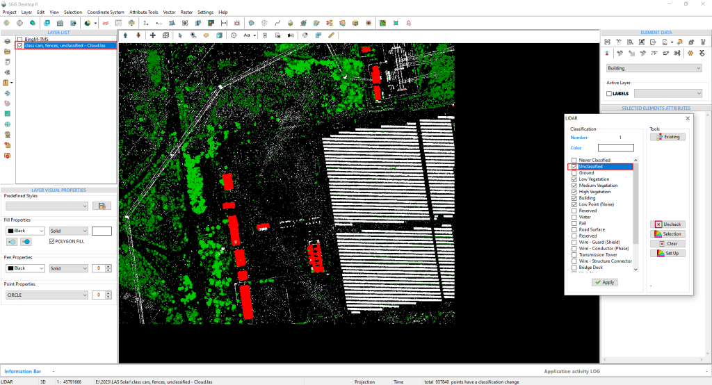
Next, we’ll enable all the existing classifications in the point cloud and click ‘Apply.’ Once the changes are applied, we can close the ‘LiDAR’ toolbox, as everything has been saved.
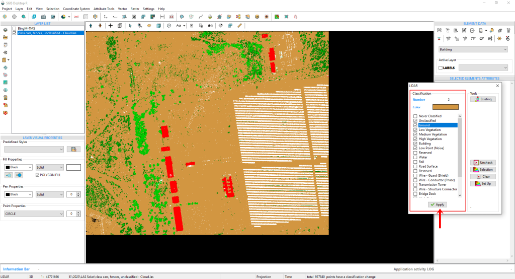
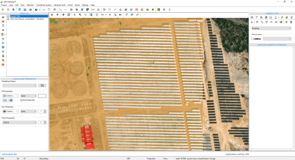
With this, the procedure is complete.
People have different visual preferences, so giving them the option to adjust the background color makes the workspace more comfortable and user-friendly. Changing the background can also enhance how LiDAR point clouds or other data are displayed, making it easier to notice small details.
For example, using a dark background might improve the contrast with lighter data points, making patterns easier to spot. Plus, staring at a bright background for hours can be tough on the eyes, and switching to a darker one can help ease that strain, especially in dim lighting.
This task is super simple—it’s just a one-click feature in SGIS, designed to give users a more comfortable experience. Let’s take a quick look at how to change the background color;
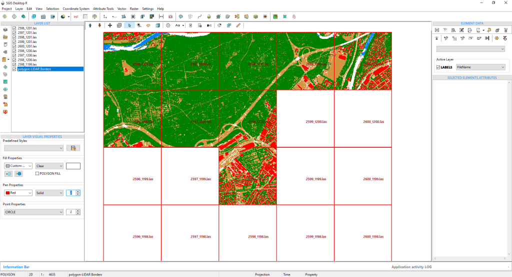
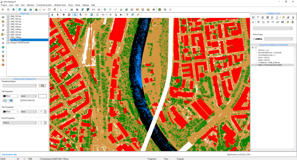
We’ve opened a LiDAR project in SGIS v.R, and the dataset includes several classifications, one of which is class 1, or Unclassified. This class contains all the man-made objects like fences, cars, and streetlights, which are typically shown in white.
Since the default background of the graphics panel is white (or light), it can be hard to see these points clearly. To fix this, we’ll switch the background to black (or dark), making the points stand out more, which will help us process the data more accurately.
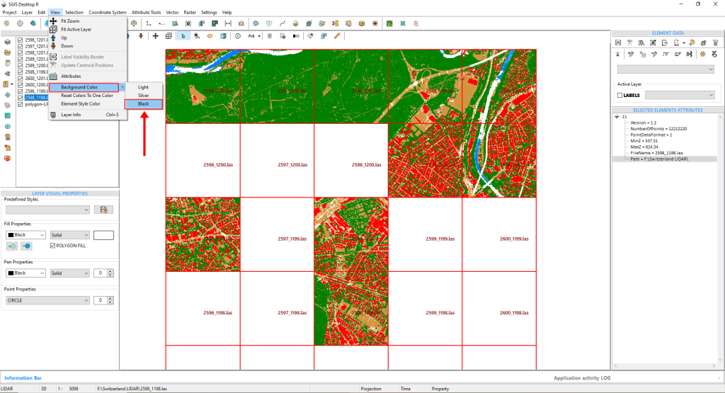
To change the background, we’ll start by going to the ‘View’ menu in the main toolbar. From there, we’ll click on ‘Background Color’, where we’ll see three options: light, silver, and black.
Next, we’ll choose the ‘Black’ option. As soon as we click it, the graphics panel will turn black, as shown in figure 108 and 109, making the LiDAR points much easier to see.
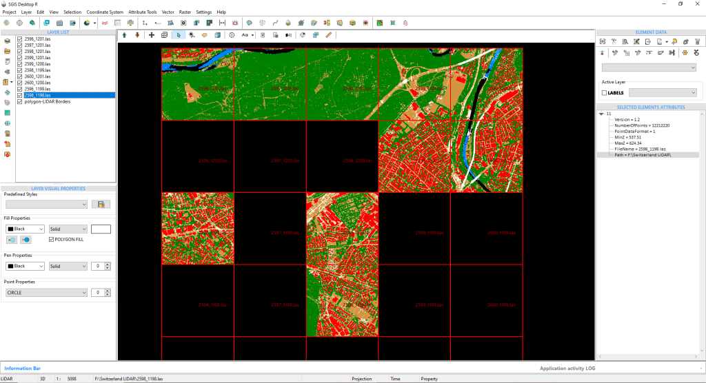
By zooming in on one of the tiles, we can see that the points are much clearer and easier to distinguish. The patterns really stand out now, allowing us to clearly identify bridges and the fences surrounding the buildings.
Additionally, if we disable the ground points, managing all the other classifications becomes significantly easier.
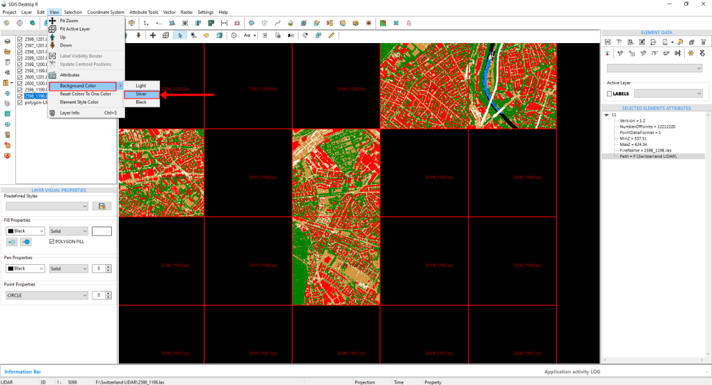
If users prefer, they can choose to switch the background to silver, which will give the graphics panel a sleek silver-gray color.
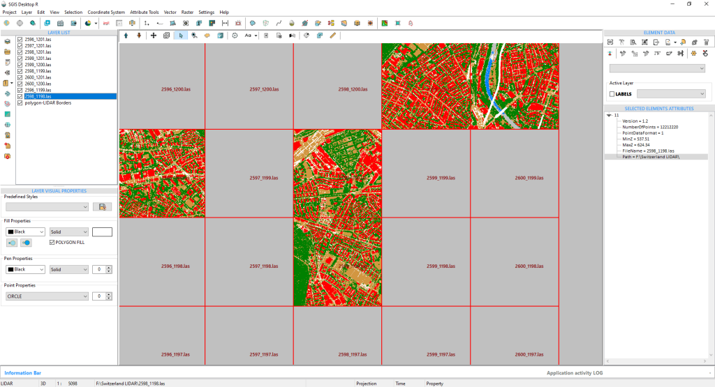
To demonstrate this function, let’s return to the main menu toolbar and head to the ‘View’ menu. From there, we’ll click on ‘Background Color’ and select ‘Silver.’
Once we do this, the color of the graphics panel will instantly change to silver-gray.
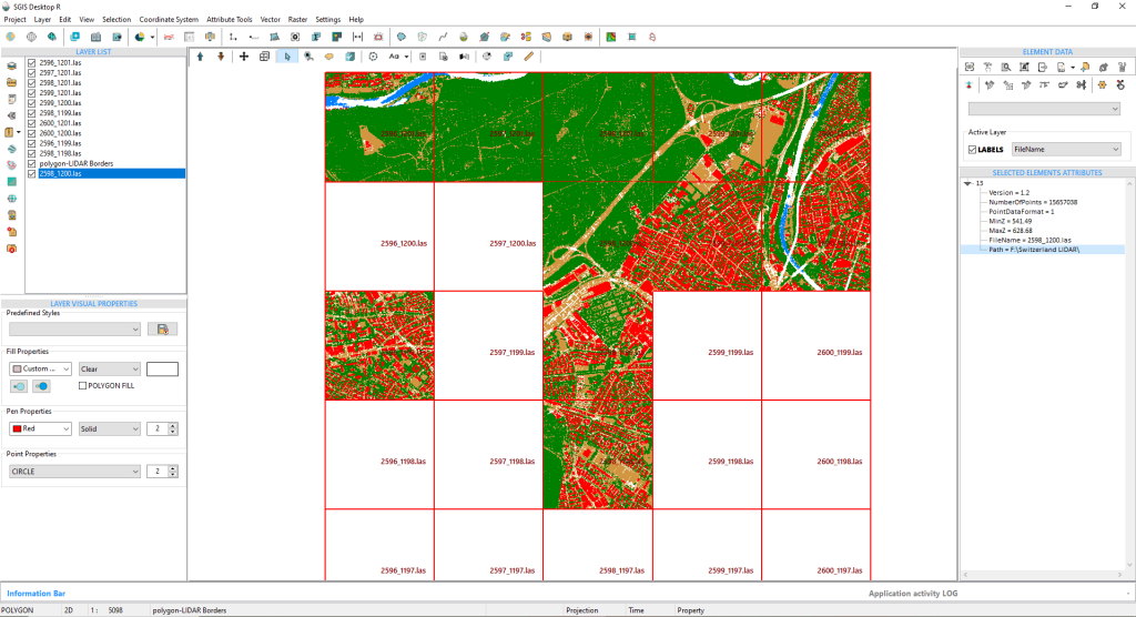
Let’s go through the procedure one more time to switch back to the default light color setting. With this step, we’ll have completed the process.
Elevation-based segmentation of point cloud data—where LAS datasets are filtered by specific elevation ranges—allows for a more targeted analysis of vertical layers within a landscape. By creating these distinct elevation bands, users can easily focus on specific vertical sections, like the ground surface, vegetation, buildings, or utility poles, which simplifies the analysis of complex terrain features.
This approach also makes data handling and processing more efficient. By narrowing in on only the relevant elevation bands for a particular task, we can reduce processing loads and focus computational power on the most critical areas, resulting in faster and more streamlined analyses.
There are many practical applications for this type of segmentation, and we’d like to highlight a few that demonstrate its practical benefits. One especially valuable use case is isolating elevation bands from LAS files for focused analysis.
For instance, we have a real-world scenario where the client needs to assess the natural slope of the terrain at a specific site to plan the installation of a sewer line. They want to connect the building to a point along the main sewer line, and by using point cloud data, we can determine the quickest and simplest route for this installation. By extracting only the ground points within the desired elevation range, we can provide the exact information needed for the task.
Another example involves extracting low-lying vegetation points from a relatively flat terrain or isolating tall building structures in an urban point cloud filled with various buildings. Each of these applications highlights the usefulness of segmentation by elevation in point cloud analysis.
We’ll demonstrate how this is done using SGIS v.R.
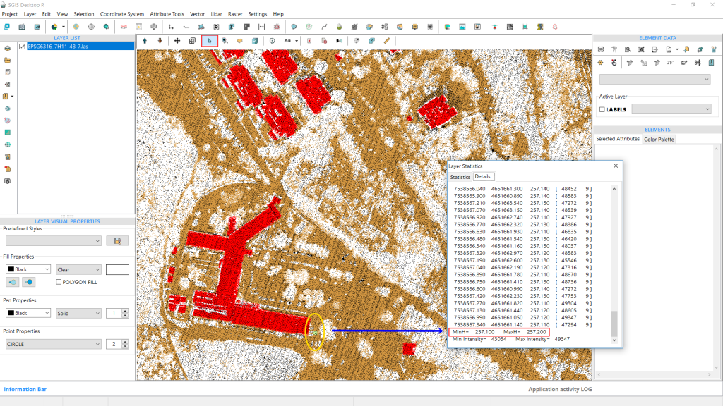
We’ve already loaded our LAS file. As shown in the graphics panel, the data includes classifications for ground, buildings, and other points marked as unclassified or class 1 according to ASPRS standards, as well as low points. This setup works well for our needs, as we’re primarily interested in the ground points for further data processing.
In SGIS v.R, the in-built ‘Statistics’ memo provides valuable data insights. Here’s how it works:
Once the LAS file is displayed, we activate the selection function. Using the mouse cursor, we click on a specific area of the point cloud at an appropriate zoom level—not too close—so we can select a group of points. By pressing CTRL+S, the ‘Statistics’ memo opens.
This memo box contains two tabs: ‘Statistics’ and ‘Details.’ We’ll open the ‘Details’ tab. Scrolling down to the end of the list, we’ll find information about minH and maxH, which indicates the minimum and maximum elevations within the selected points. This tells us the elevation range for that particular cluster of points.
With this elevation data, we’ll know the exact range to input in the ‘Elevation Range’ selection process. In our case, we’ll take note of 257.5m H and move forward with processing.
Next, we’ll close the Statistics window. Below the ‘Element Data’ toolbox, there’s a dropdown menu displaying various classifications. From here, we’ll select “Ground” points. This means that any selection procedure or function we apply will target only the ground points, not the entire point cloud. If we had chosen class 1, for instance, the selection would focus specifically on those class 1 points instead.
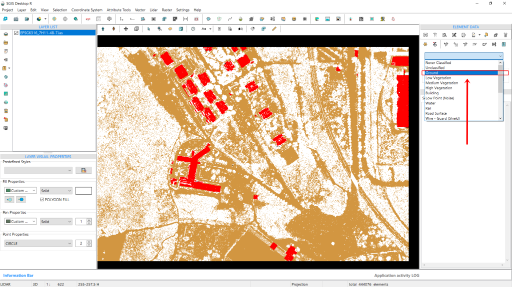
Next, we’ll navigate to the Selection menu and choose ‘Select Elements by Elevation Range’.
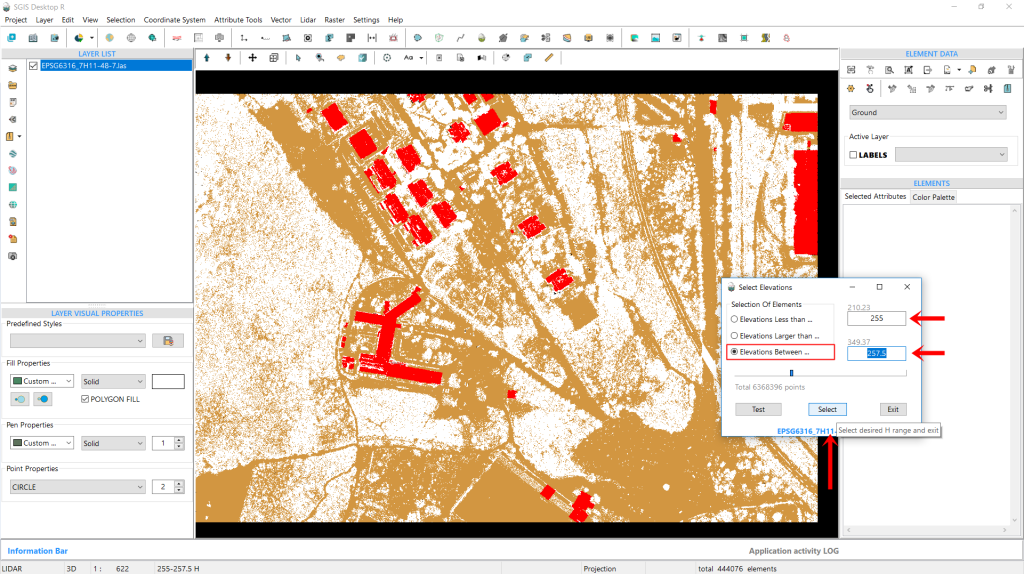
Then, we’ll check the third box labeled ‘Elevations between…’ As soon as we click on this option, the input boxes on the right become active. In the first box, we’ll enter H 255 m, and in the second box, we’ll enter H 257.5 m. This setup means we want to highlight and select all ground points with elevations ranging from 255 to 257.5 m.
Finally, we’ll click on ‘Select’ to proceed.
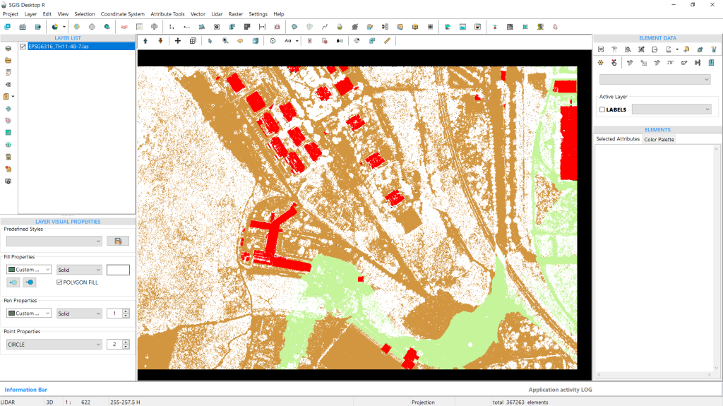
As shown in Fig. 116, all the points that meet this criteria are now selected and highlighted. For clarity, it’s important to mention that we previously changed the highlight and selection color to green. The default red color wasn’t suitable for several other previous projects, where we needed to highlight buildings that were also red.
This is a customizable option that users can modify according to their preferences.
Next, we’ll use the ‘Selected Elements in New Layer’ function to separate these points into a new layer, which we’ll name “points 255-257.5 H.” If we create multiple layers for different elevation bands in the Layers panel, giving them clear names will help us keep track of everything during our processes.
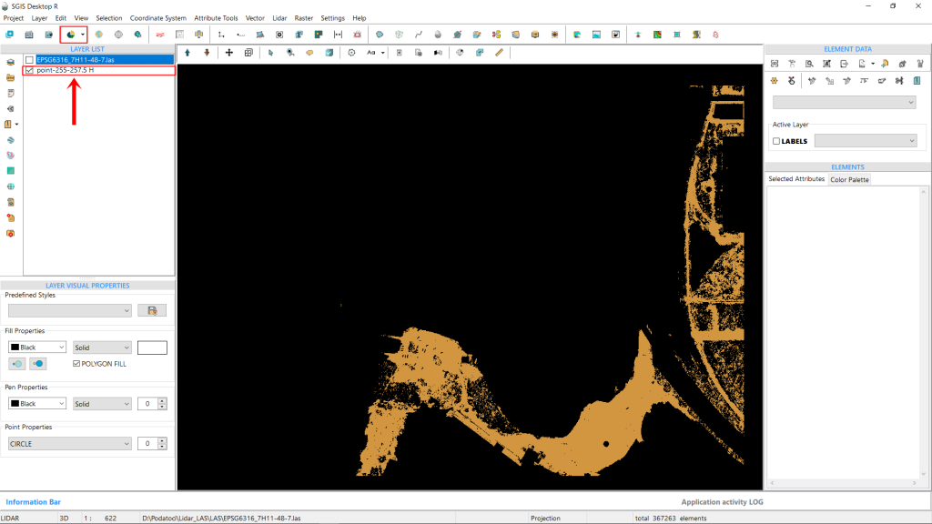
This extracted point dataset can later be saved as a separate LAS file, or in TXT, CSV, ASCII, or XYZ formats. In our specific case, this means we have the ground elevations from the desired point A to point B, allowing us to create profile sections and conduct further analysis. Additionally, since this dataset contains significantly fewer points than the entire point cloud, it reduces the strain on hardware during subsequent processing.
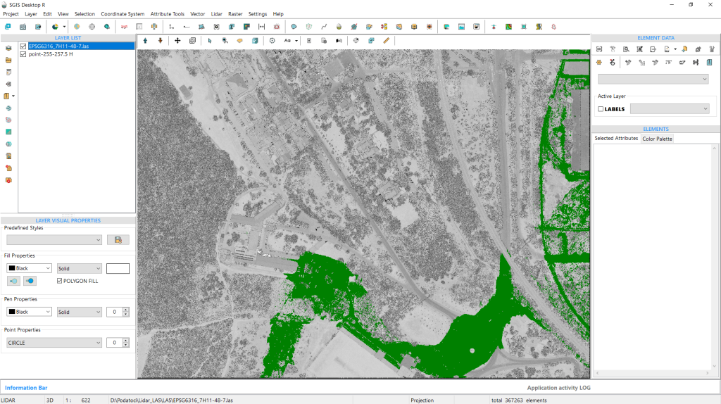
To get a clearer view, we’ll enable both layers from the Layers panel. The first layer will display the entire point cloud, which we’ll set to Intensity view mode. We’ll also change the color of the extracted ground points for better visibility.
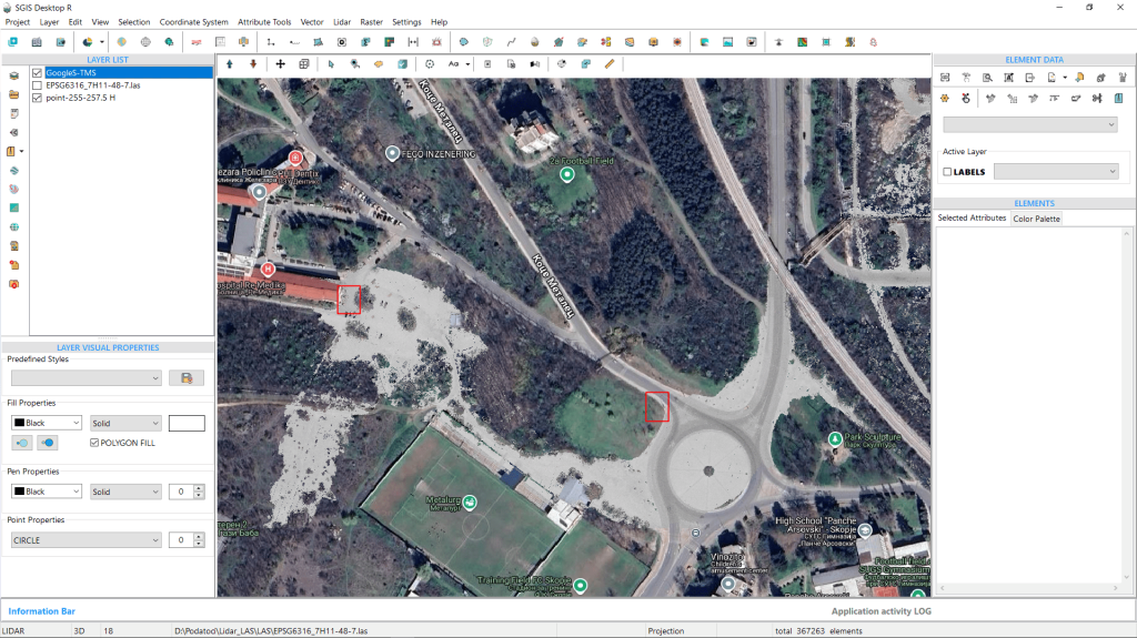
Alternatively, we can disable the entire LAS point cloud and add a Tile map layer as a backdrop, showing only the extracted points in Intensity view mode. This approach, illustrated in Fig. 119, is particularly useful because the intensity view allows us to clearly see features like roads and concrete surfaces.
We’ll look at another example from a practical case with an urban point cloud. This LAS file includes multiple structures, such as houses and buildings, among which are three tall buildings that we’re focused on extracting for this example. Since this area is densely built, we need to carefully examine the elevation data to isolate the tallest buildings.
The point cloud has been imported, and we’ve already set the classifications using the ‘LiDAR’ toolbox. After reviewing the available classifications, we found only Ground, Unclassified, and Low points in this dataset. We’ve disabled all points except for classification 1. Since vegetation (low, medium, and high), unclassified points, and building points are all included under class 1, we first need to assess the elevation in our target area.
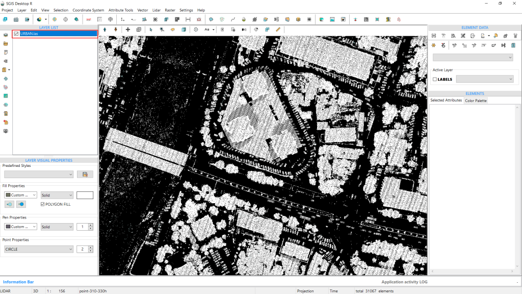
So, we’ll repeat the process by selecting clusters of points at several spots. Then, we’ll press CTRL+S, go directly to the Details tab, and scroll to the bottom to view the minH and maxH values. We’ll repeat this once more to ensure a precise elevation check.
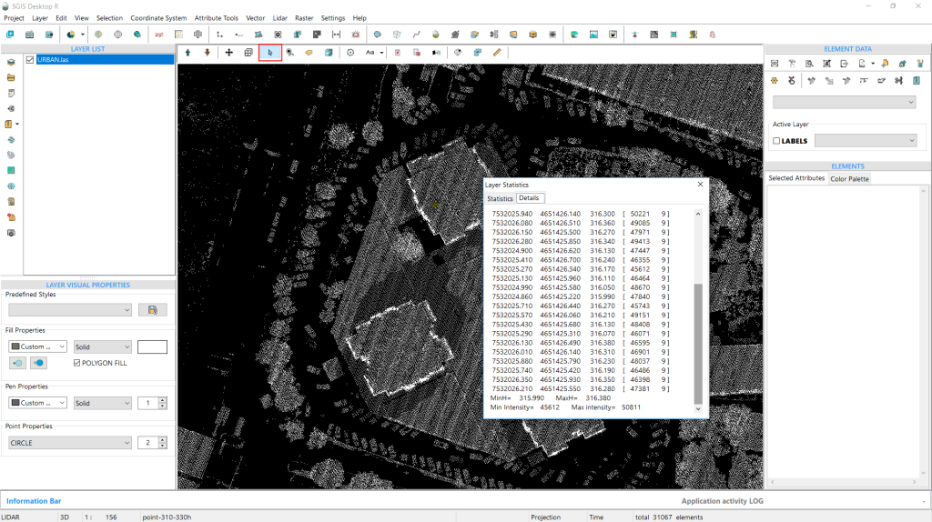
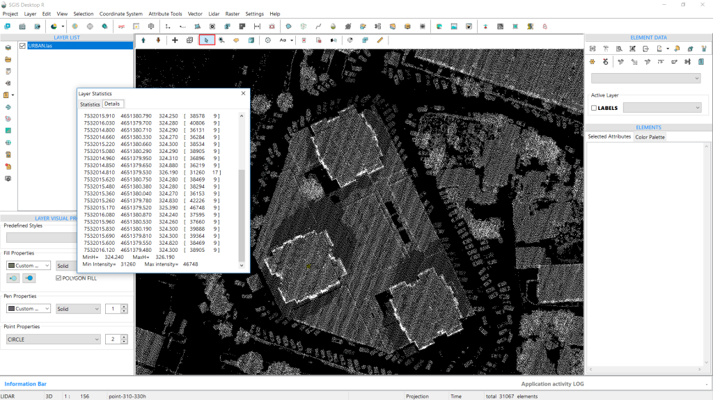
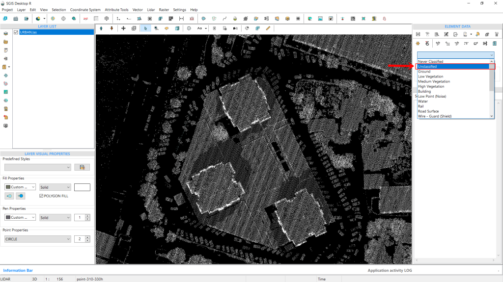
Once we’ve noted the necessary elevation values, we open the classification dropdown on the interface and select “Unclassified,” as we’ll be working with points from this classification. Next, we navigate to the Selection menu and choose “Select Elements by Elevation Range” once again. A dialog window appears, prompting us to set the parameters. We check the box labeled “Elevation Between…” and enter the desired elevation values. This time, we’ll specify a range from 310m to 330m. With these values in place, we click “Select” to continue.
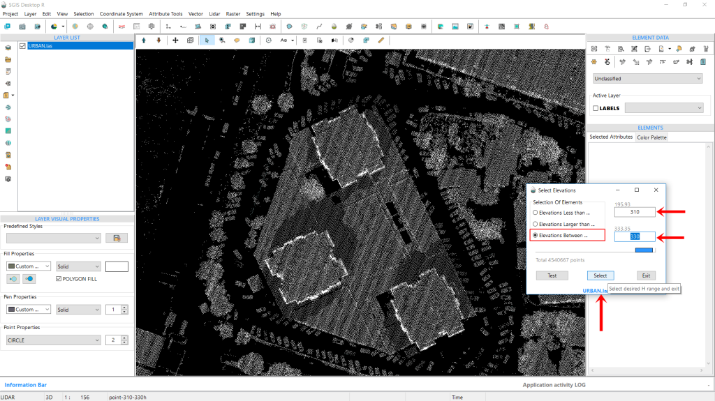
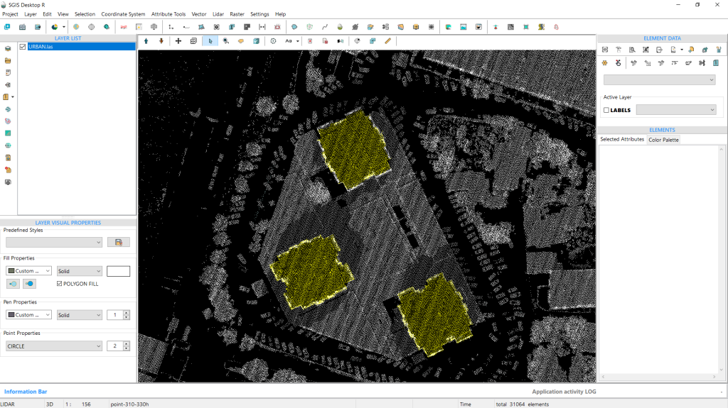
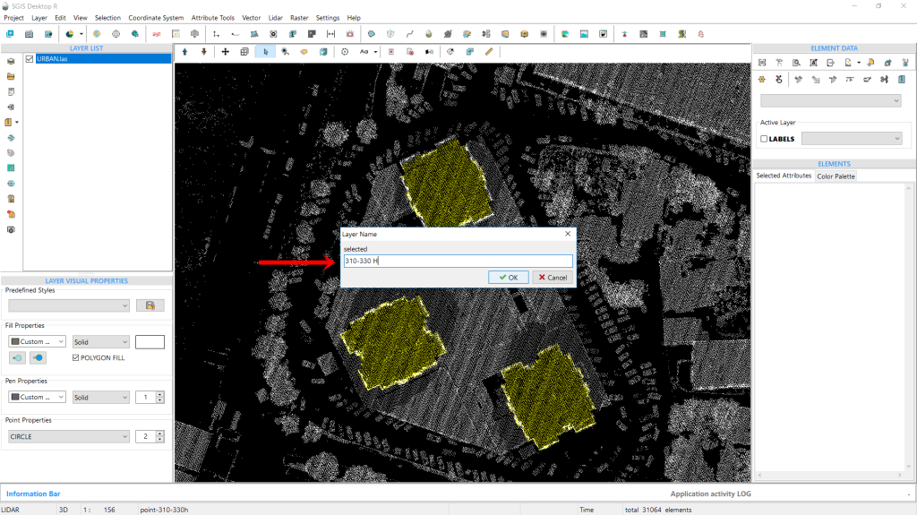
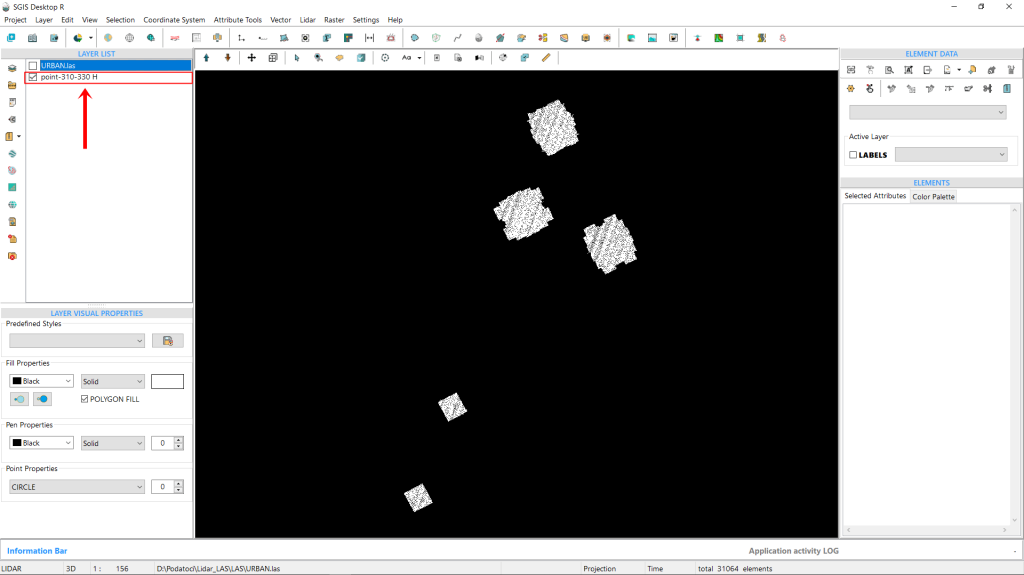
The points are instantly selected and highlighted in a bright yellow color. Next, we’ll isolate these points into a new layer using the ‘Selected Elements in New Layer’ function. When prompted, we’ll name this layer “points 310-330 H” to ensure clear distinction for future processing. After entering the name, we click ‘OK’ to create the layer.
When we zoom out, we can see that, in addition to the three buildings we were targeting, two more buildings also fall within this specific elevation range. Since we don’t need these additional buildings, we can easily select and delete them. This is worth mentioning since we are selecting points from a specific ASPRS classification, but we’re still working with the entire point cloud. With that, we’ll wrap up our procedure.
Intensity in LiDAR data refers to the strength of each laser pulse’s return signal when it bounces back from a surface.
This strength can vary depending on the reflectivity of the object hit by the laser, which in turn depends on factors like the material’s properties and the wavelength of the laser—usually in the near-infrared range. For instance, different materials (like concrete, vegetation, or metal) reflect light differently, so their intensity values will vary.
In LiDAR processing, intensity values play an important role in identifying and categorizing features within a dataset. It’s often used to support feature detection, point classification, and sometimes even as a substitute for aerial imagery when those aren’t available.
Since intensity values are relative (rather than absolute), they can change based on factors like flight height or environmental conditions. This means that the intensity recorded for the same target might differ from one flight to another.
SGIS v.R is enhancing this capability by offering tools to generate intensity-based images directly from LiDAR data. Users will be able to seamlessly switch between classification and intensity views while working, adding a new layer of detail to their analysis.
This flexibility can be especially valuable, providing clearer insights into surface characteristics and improving the precision of feature detection.
What Is the Purpose of Intensity in LiDAR Processing?
Intensity values are valuable because they allow you to visualize point clouds in a way that highlights the reflective properties of different surfaces.
For instance, materials like asphalt tend to show up with lower intensity (darker), while metals and vegetation often display higher intensity (brighter). This contrast makes it easier to differentiate between materials and identify vegetation, which is particularly useful in fields like urban planning and forestry.
This makes intensity data especially useful for tasks like land classification, object recognition, and enhancing digital surface models. Intensity-based images also aid in feature extraction, making it easier to classify various surfaces, such as roads, buildings, and vegetation.
This demonstration will outline how to visualize LiDAR data by intensity using SGIS technology in SGIS v.R through a couple of practical examples. First, a LAS dataset is imported using the ‘View LiDAR Boundaries’ tool. Subsequently, the ‘LiDAR’ toolbox is accessed.
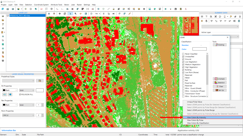
In the ‘Tools’ tab, users will find various buttons designed for managing LiDAR point cloud data, whose functions and purposes have been previously described. Therefore, we will proceed directly to this functionality. After navigating past the ‘Set Up’ button, a blank memo space appears. By right-clicking in this space, a new dropdown menu will appear. Here, users can find options for managing, selecting, and visualizing points. The data can be visualized not only by classification but also by intensity and pulse range. Additionally, users can make selections based on intensity values and pulse range. These functions will be explained in detail in another practical use case example.
As this is an ongoing development, these functions may be located in different areas of the software or may appear slightly modified in the final version. Nevertheless, our focus is on describing the technology and its valuable practical applications.

In the new dialog menu, navigate to ‘View Colors by Intensity’ and select it.
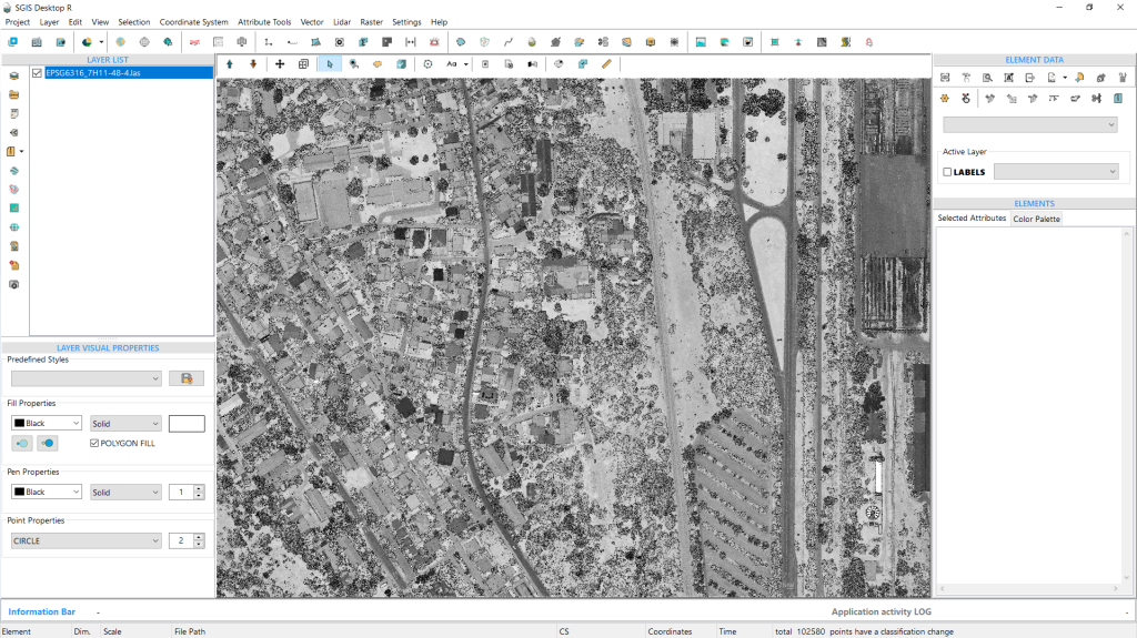
Once selected, the points will be displayed according to their intensity values. This view serves as an alternative to traditional aerial imagery datasets. When standard aerial imagery is unavailable, intensity-based LiDAR images can provide a suitable substitute. These images resemble black-and-white photographs and offer essential visual information for further processing and analysis.

We will include another example from an urban setting featuring roads, buildings, vegetation, and man-made objects.
By analyzing intensity values, LiDAR data can be utilized to categorize and detect objects, as well as enhance the differentiation of surfaces, particularly concrete surfaces such as roads and various types of buildings.
A color hillshade is an elevation map that blends shaded relief with color gradients, providing a vivid depiction of terrain. By combining shadows and colors, it enhances the perception of depth and reveals intricate details of topographic features.
By ‘Direct Color Hillshade Creation,’ we mean an efficient way to generate colorized hillshade DEMs directly from a LAS file (by interpolating point data), from an ASCII DEM (Digital Elevation Model) file, or any active GIS layer with elevation data (such as DEMs, for e.g., in TIFF format), without requiring extra steps like file conversion or multiple styling processes.
With SGIS, we’ve simplified the process to make it much easier for users. We’ve made it possible for users to open a LAS file and directly interpolate a color hillshade DEM, or load an ASCII DEM, select an elevation-based color ramp, and let SGIS automatically generate the colorized hillshade DEM, which can then be exported as a DEM or a raster image file (georeferenced raster image file). There’s no need for multiple styling steps or blending modes—just one step, and the color hillshade is ready.
We’ve made this available through several loading options, and we’ll demonstrate some of them with practical examples.
Enhancing Terrain with Color
Color gradient (elevation-based) hillshade DEMs are a way to visualize terrain by combining shaded relief with color gradients that reflect elevation levels. This technique gives a clear and detailed representation of the landscape, enhancing our understanding of both its depth and elevation variations.
Hillshading simulates shadows and highlights, as if the terrain is lit from a particular angle, which helps to reveal the contours of slopes, ridges, valleys, and other landforms. Along with the shading, colors are applied according to elevation, with different colors indicating different height ranges. For instance, lower elevations might be shown in shades of green and brown, while mid-elevations could use yellows, and higher elevations may appear in whites or blues.
By combining the hillshade effect with these color gradients, the final image provides a clear and intuitive view of the terrain’s structure and elevation changes. This makes it easier to interpret the landscape as a whole. Color gradient hillshade DEMs are especially valuable in fields like:
- Geology and Environmental Studies: Useful for analyzing landforms, watersheds, and erosion patterns.
- Urban and Land Use Planning: Helpful for identifying suitable construction sites, assessing slopes, and planning infrastructure.
- Cartography and Visualization: Effective for creating engaging maps that are easy to understand.
SGIS v.R Technology
The simplest approach we provide with SGIS technology is to check the “Create Color Hillshade” box during the interpolation of a point cloud, which will automatically generate the hillshade.
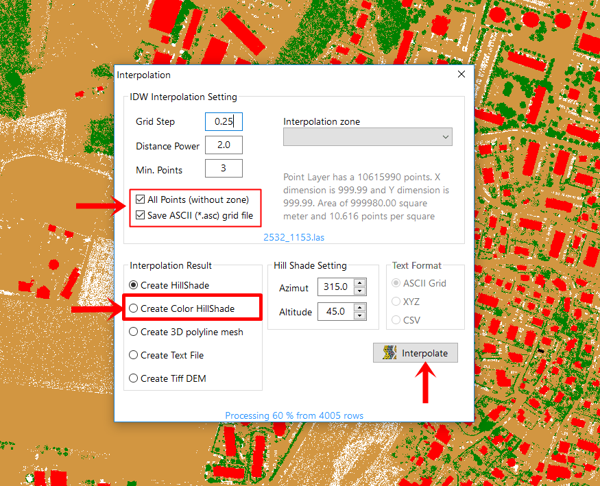
But, we also want to showcase additional options by providing practical examples that highlight the capabilities of SGIS v.R.
To demonstrate this, we loaded a LiDAR boundary grid, which will allow us to add a LAS point cloud.
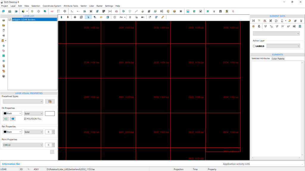
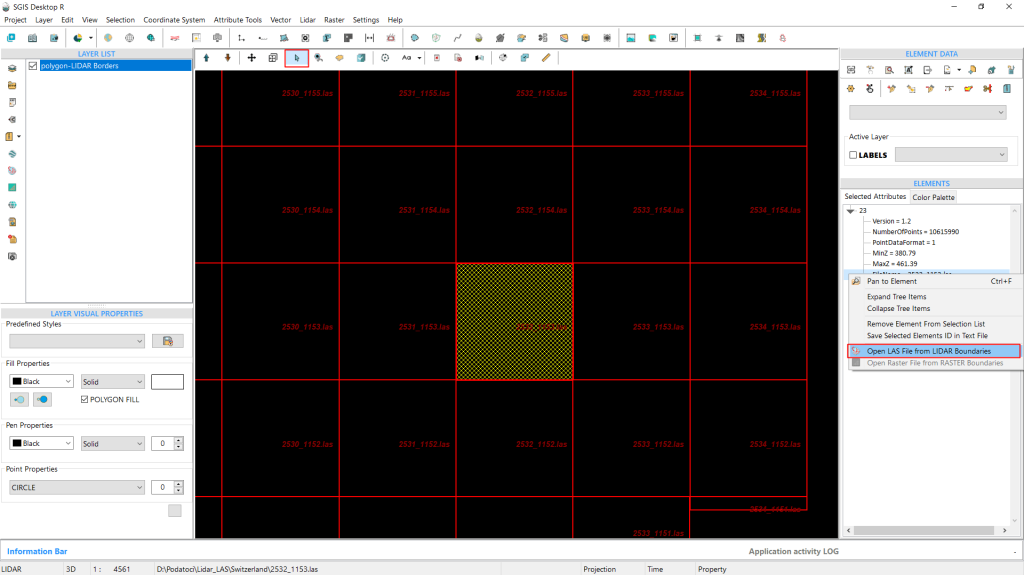
We styled the LiDAR boundary grid earlier to show the file names, making it easier for us to understand and locate our data.
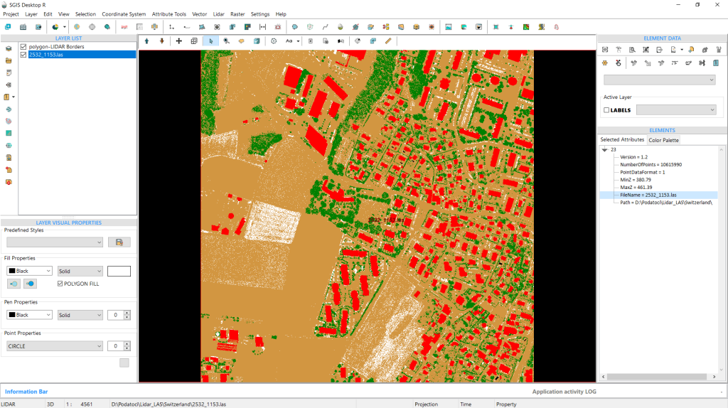
We also changed the background to a darker color. Now, we can select the desired LAS file and right-click on a row from the ‘Elements’ toolbox to open it.
The LAS point cloud is loaded right away.
Next, we’ll adjust the interpolation parameters. We’ll set the Grid Step to 0.25m, the Distance Power to 2, and the Minimum Points to 3. Additionally, we’ll check the boxes for ‘All Points’ and ‘Save ASCII’, which we’ll explain further along in the process.
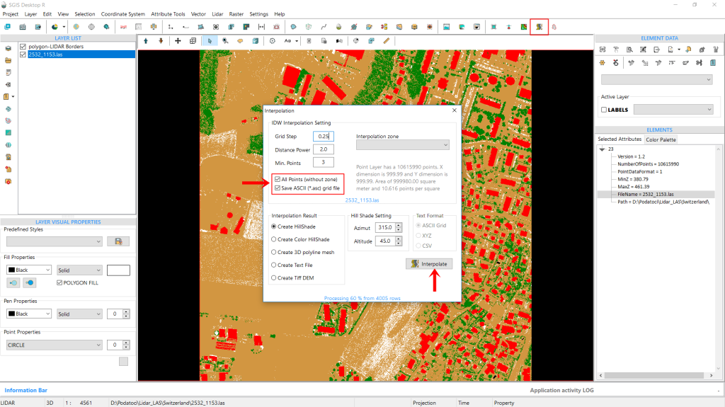
We’ll also keep the default setting for ‘Create Hillshade’ in the Results tab. Once everything is set, we click on ‘Interpolate’.
We’ve detailed this process in our document titled “[Developing Algorithm for Creating a DEM Grid from LiDAR Point Cloud Based on IDW Spatial Interpolation in SGIS v.R – Interpolating LIDAR Point Clouds to Raster with IDW with SGIS v.R].” The outcome of this interpolation is the generation of the hillshade DEM, which is reflected in the new layer that appears instantly in the ‘Layers List’ panel.
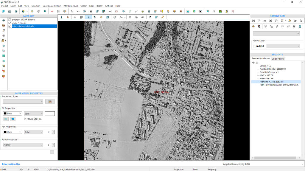
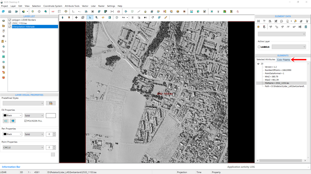
Now that we’ve completed this step, we’ll move to the ‘Color Palette’ tab under the ‘Elements’ panel.
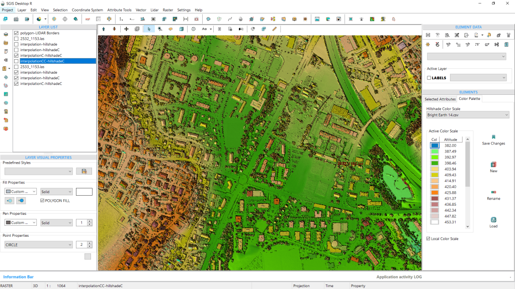
This tab offers a visual color scale ramp, as well as several other tools. We’ll start with the ‘Hillshade Color Scale’ dropdown, where we can select a preferred color scale. SGIS includes multiple preset color ramps, and users can also add custom color scales. In Fig. 139, we see a preset called ‘Earth Tone 5,’ which consists of five colors, each adjusted to specific elevation values displayed below the dropdown.
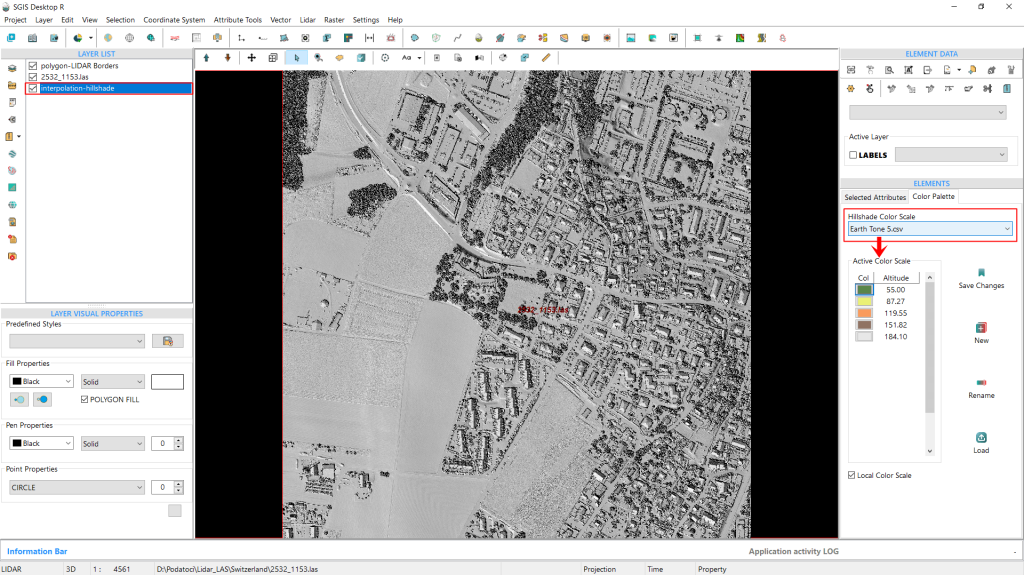
To demonstrate the simplicity of this feature, we’ll leave the color scale as-is, using the default ‘Earth Tone 5’ preset. For users working with a preloaded DEM-hillshade without a LAS file, SGIS provides this second option to create a Color Hillshade directly from the ‘Raster’ menu by simply selecting a preset color scale.
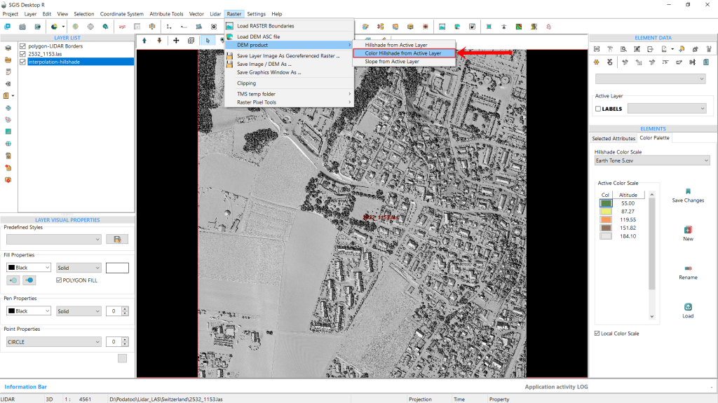
Since we’ve now completed the creation of our example hillshade process, and the hillshade layer is visible in the ‘Layers List’, we’ll navigate to the Raster menu, go to ‘DEM Products’, and select ‘Color Hillshade from Active Layer’. Clicking on this immediately generates the color hillshade as a new layer in the Layers List.
Additionally, users can choose to display their data with either a local or global elevation scale. In our example, we’ve used the local scale option, which provides a tailored representation based on our specific terrain. This new color hillshade DEM layer reveals a clear contrast to the regular hillshade, making it easy to identify variations in elevation.
With color, it’s much easier to distinguish high and low areas, enhancing both depth and elevation, and terrain detail.
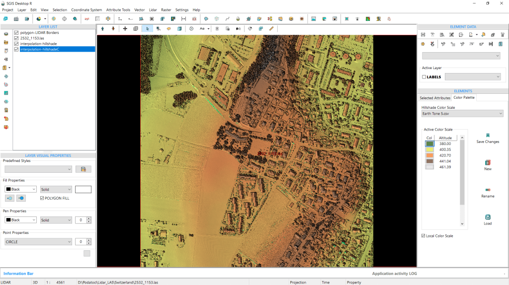
The color hillshade is now generated, and its layer appears in the Layers list.
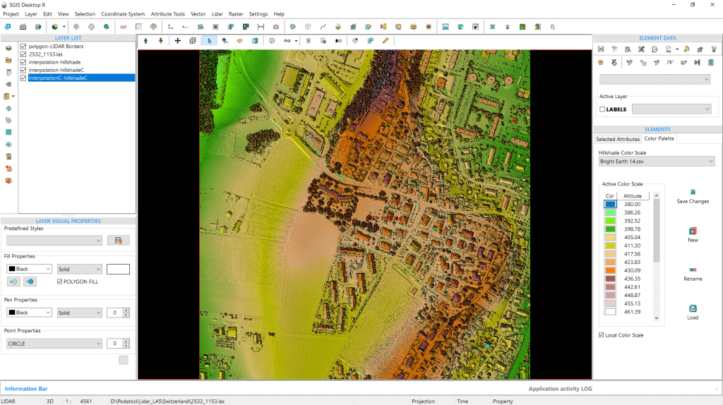
If we want to change the color scale, we can easily do so by opening the dropdown menu and selecting a different preset. For this example, we’ll select the ‘Bright Earth 14’ palette. The “14” here represents the number of elevation intervals in the preset, meaning it uses 14 distinct colors to represent varying elevations.
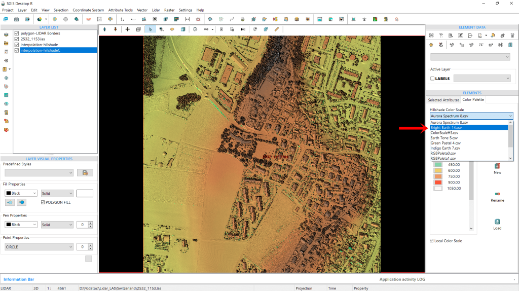
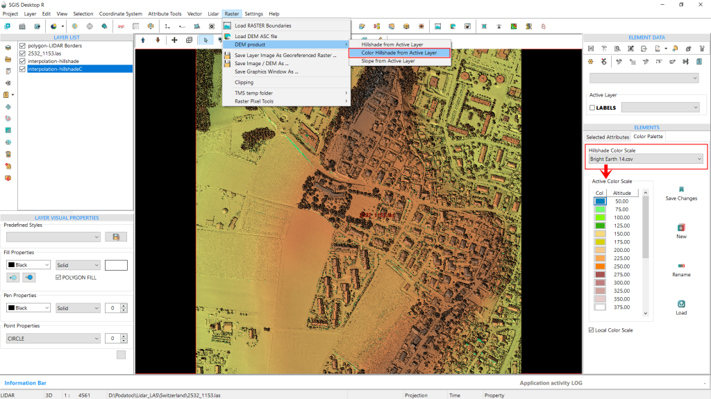
To apply the change, we simply need to select the desired preset from the list and then click on the ‘Color Hillshade from Active Layer’ option again. This action will create a new color hillshade layer, which will appear in the list of layers.
This updated representation provides a more intuitive view, showcasing the elevation changes in the terrain with greater detail.
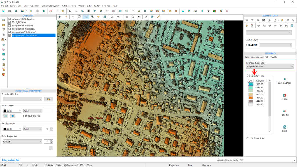
To highlight some of our presets, we’ll go through the process again, this time using the ‘Indigo Earth 7’ color hillshade scale. The outcome of this selection is displayed in Fig. 145.
We’re going to repeat the entire process to highlight the potential benefits for users working on large-scale projects that involve multiple LAS files, or DEMs (DEM hillshades). By demonstrating how colorizing hillshades according to their elevation values enhances terrain visualization, we aim to show just how much more intuitive and informative the resulting maps can be.
To accomplish this, we’ll choose the LAS file that is adjacent to the one we’ve already processed. First, we select the LiDAR boundaries layer, then click inside the grid square. After that, we can right-click to open the submenu and load the LAS files from there.
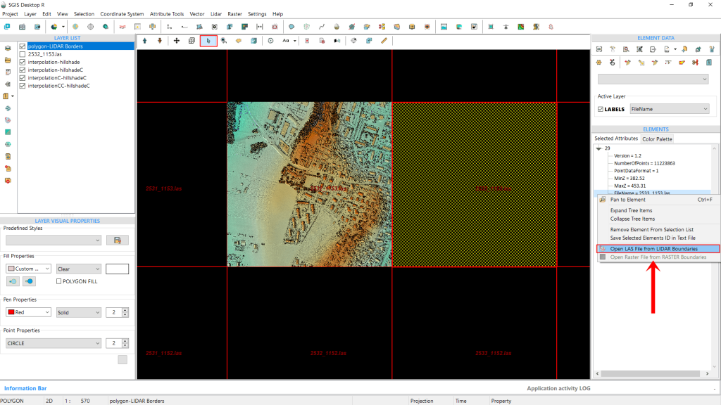
To make the process quicker, we’ve already created the hillshade. Now, we simply need to select the same ‘Indigo Earth 7’ color scale palette for both layers so they visually blend together (HS DEM 1 and HS DEM 2).
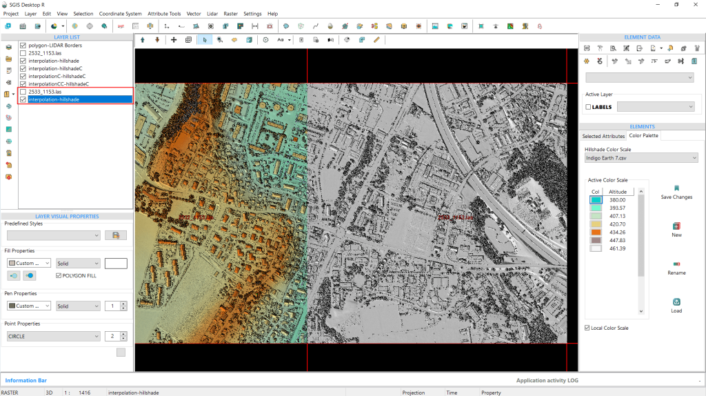
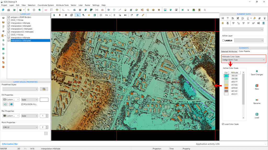
In Fig. 148, we see the smooth transition and seamless blending of both DEMs into a single, cohesive image, offering a vivid representation of the terrain.
The elevation color ramp shows the lowest areas in indigo blue, with elevation gradually increasing toward the left and right sides. This detail is far more discernible than with a standard gray hillshade.
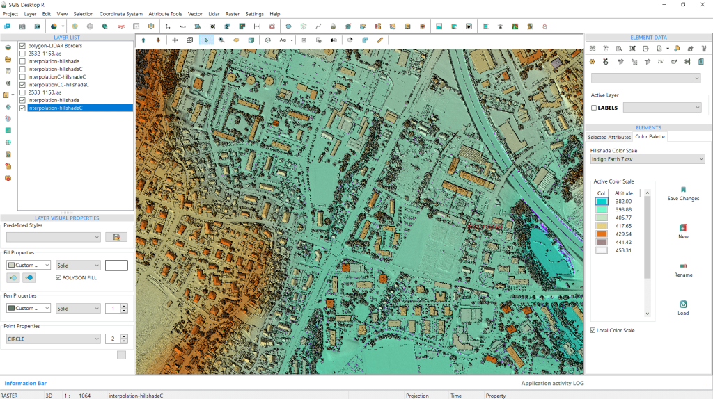
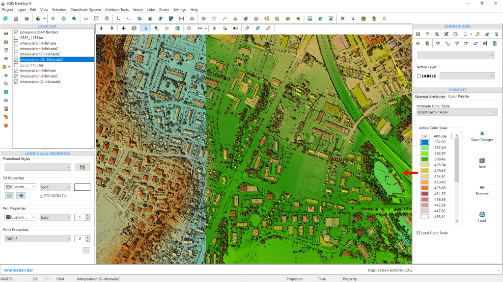
We can also adjust the color ramp for one DEM hillshade while keeping the original for the other, or modify both for a cohesive visual effect. Using a different color ramp allows for a more nuanced depiction of elevation changes, enhancing terrain detail.
We’ll demonstrate now how to create a color hillshade DEM by directly loading an ASCII DEM file (.asc grid file) into SGIS v.R.
An ASCII DEM (Digital Elevation Model) is a type of file format that presents elevation data in a simple text form. The term “ASCII” refers to the American Standard Code for Information Interchange, indicating that the information is stored using standard text characters. These files usually contain geographic coordinates along with elevation values arranged in a grid format. Each line represents specific elevation data points, collectively creating a digital model of the terrain.
In GIS applications, ASCII DEM files are frequently utilized for tasks such as terrain analysis, visualization, and generating models like hillshades. Their text-based format makes them easy to read and compatible with a variety of software platforms.
That’s why we checked the ‘Save ASCII’ checkbox in the interpolation dialog window earlier. If users have a LAS point cloud and want to save the data in a more shareable DEM Grid format, they can easily do so while generating the hillshade with those settings translated into the ASCII DEM Grid as well. The ASCII file will automatically be saved in the same folder as the original LAS data files, making it convenient to access and share.
Since using the exported dataset would yield the same results as before, we’ll use a different .asc file for this demonstration. This will allow us to explore the additional tools available in the ‘Color Palette’ tab.
We’d also like to explore the creation of colored hillshade for undulating terrain with mixed forest cover.
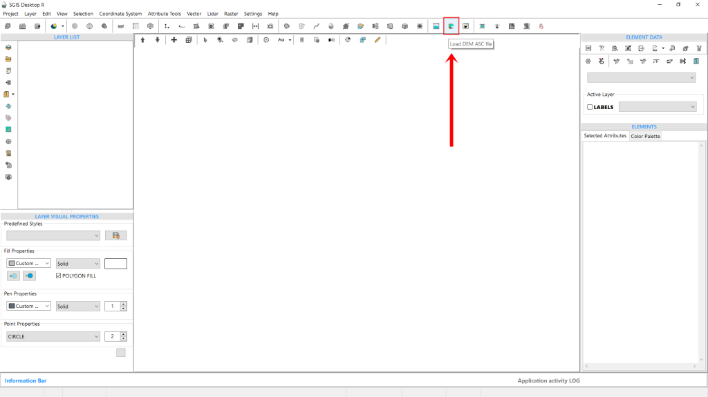
Let’s begin by locating the ‘Load DEM ASC file‘ function, conveniently placed in the main ribbon bar of the software interface for quick access.
After selecting it, a new dialog window opens, prompting us to configure some settings for our task. First, we’ll define the file path to locate our desired DEM file.
Then, we’ll set the ‘Mode’. Currently, there are four modes to choose from:
- Two-Color Shade;
- Color Scale;
- Contour Lines;
- and Hillshade.
We’ll walk through each mode with practical examples later, but for now, we’ll stick with this demonstration and select the fourth option by checking the ‘Hillshade’ checkbox.
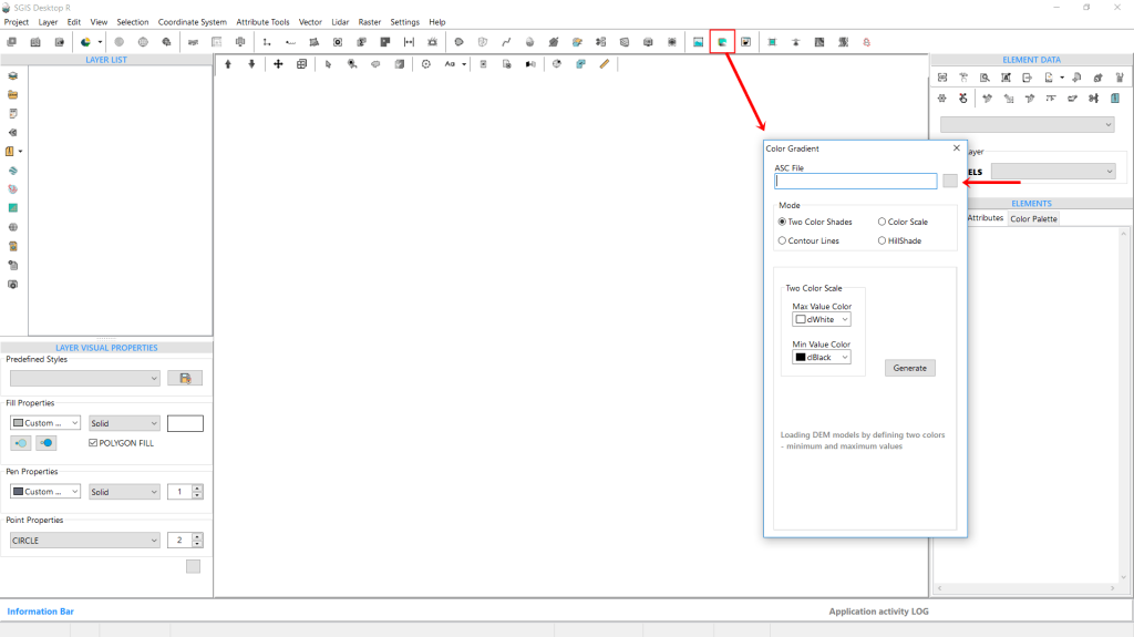
Comparing Fig. 153 and Fig. 154, we can see that by default, the function opens with the ‘Two-Color Shade’ mode selected. However, when we switch to Hillshade by checking its box, the menu adjusts to show new options. In the original view, users can adjust settings specific to ‘Two-Color Shade,’ but with Hillshade selected, the “Result” box offers three options:
- Hillshade,
- Color Hillshade,
- and Slope.
For this example, we’ll select Color Hillshade.
Below this, additional hillshade settings for Azimuth and Altitude appear, set by default to 315° and 45° respectively. With everything configured, we just need to click ‘Generate’ to complete the process.
The color hillshade DEM is instantly created as a new layer and displayed in the graphics panel.
Notably, we previously set the color scale palette to ‘Indigo Earth 7,’ so the software automatically applies this palette as the default for any new color hillshades generated unless it’s changed.
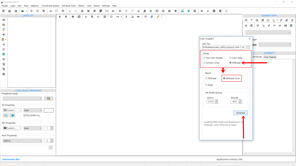
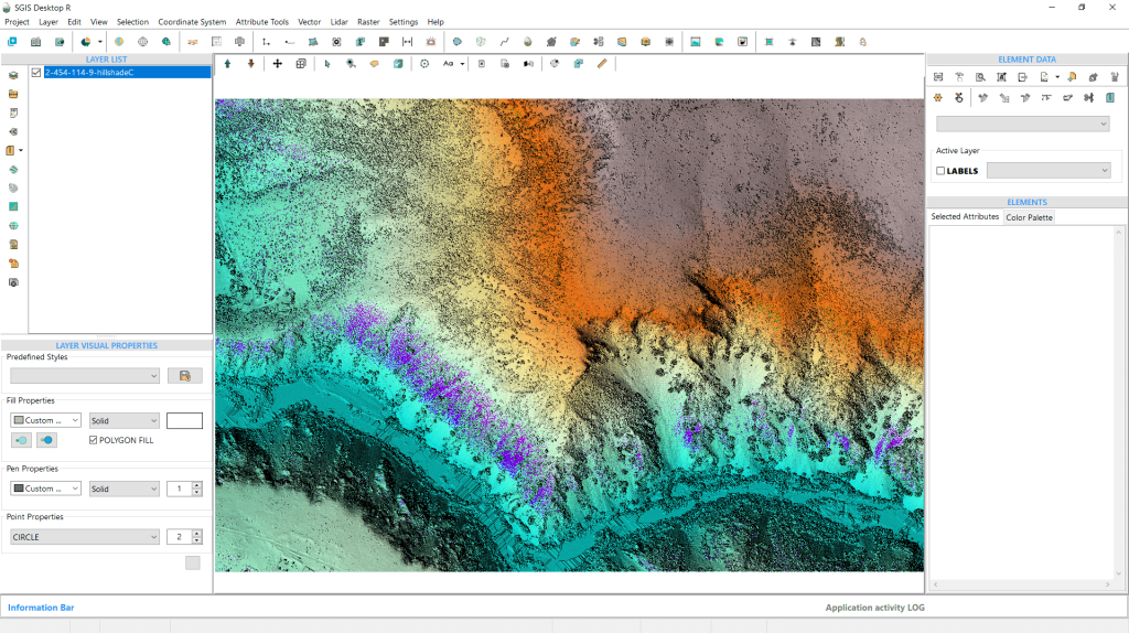
We’d also like to go over the tools available in the ‘Color Palette’ tab, which allow users to adjust and manipulate color scales for enhanced visualization.
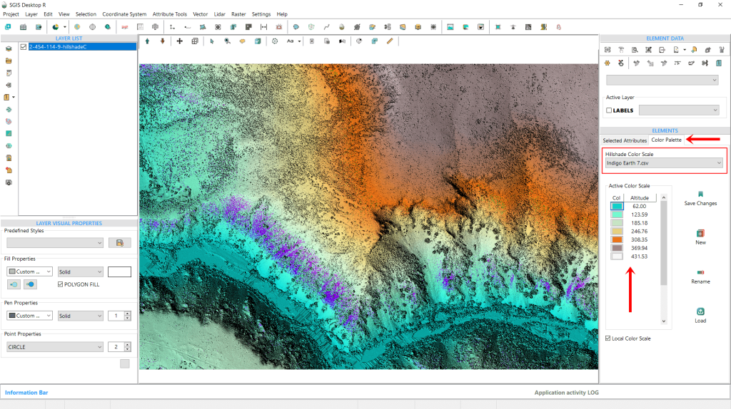
Earlier, we covered how to change the color scale by selecting from the dropdown list, which includes some preloaded SGIS presets. However, users can further customize the color scales using the tools on the right side of the toolbox. Let’s now go over each of these tools in detail.
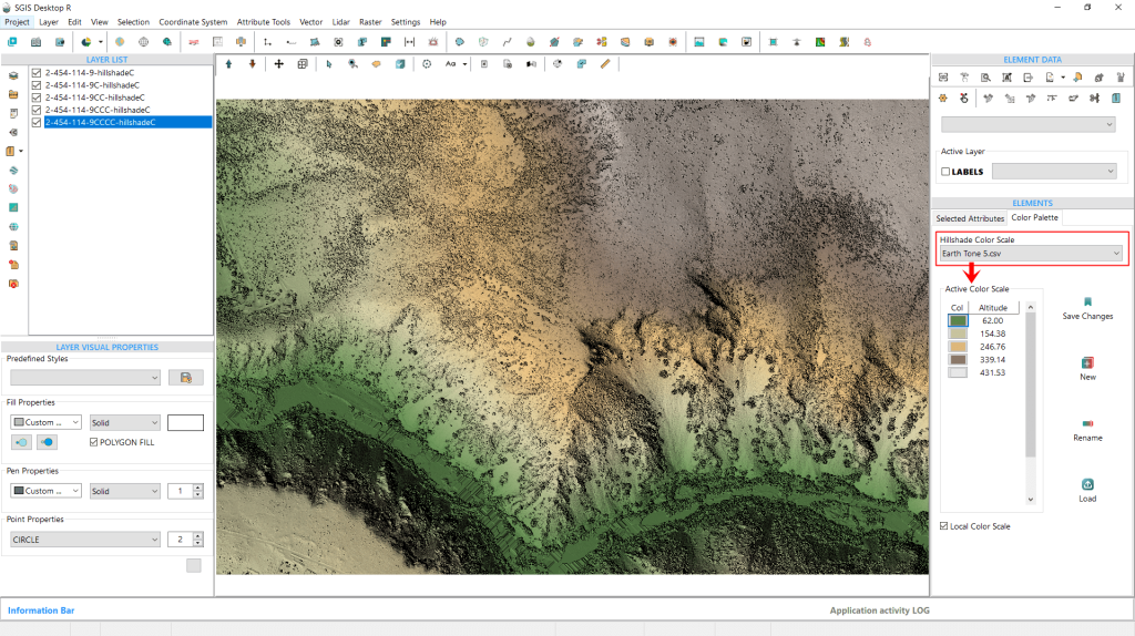
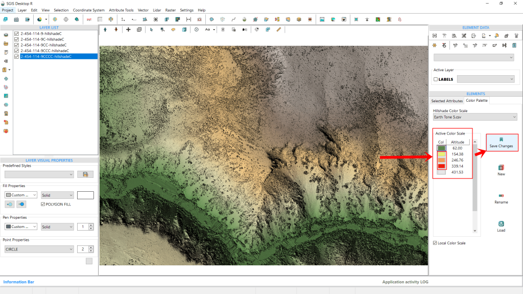
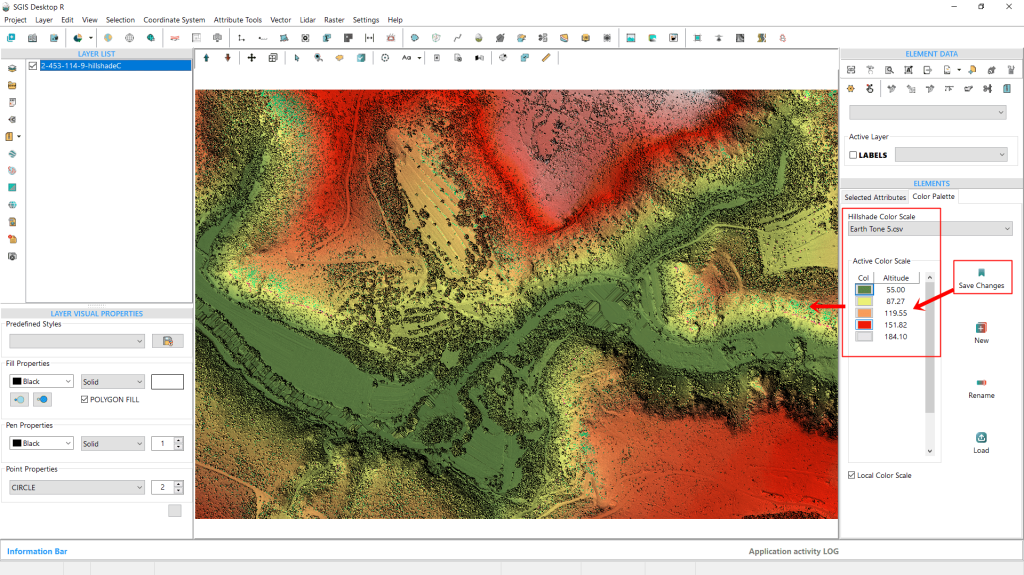
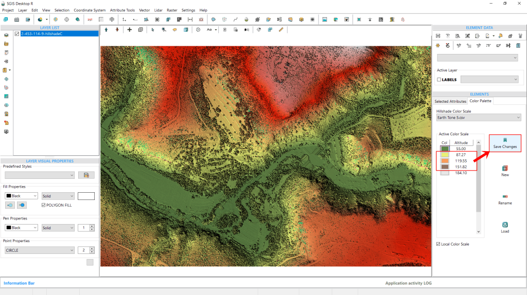
We’ve changed the preset, as shown in Fig. 157, selecting one with fewer elevation intervals, ‘Earth Tone 5.’ In this view, we can also see the color values assigned to each elevation interval. To modify these, simply click on the color rectangle. A color palette will pop up, allowing us to pick a new color for that particular elevation.
For this example, we’ve decided to update the colors of the three middle elevation values within the ‘Earth Tone 5’ scale. To save these changes, all we need to do is click the ‘Save Changes’ button on the right side.
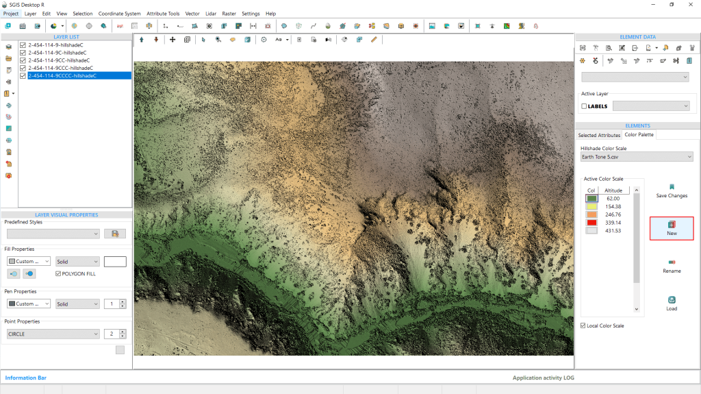
The next function, ‘New’, lets users create a custom preset by entering minimum and maximum elevation values in a dialog window and specifying the number of intervals they want for the custom scale.This new scale will then be available for future use in the dropdown list for further analysis.
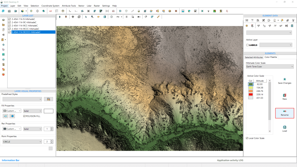
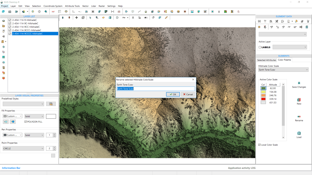
The third option is the “Rename” feature, which allows users to rename color scales for better organization and personalization. This is particularly useful for customizing presets, enabling users to give them names that are easier to remember or align with their preferences.
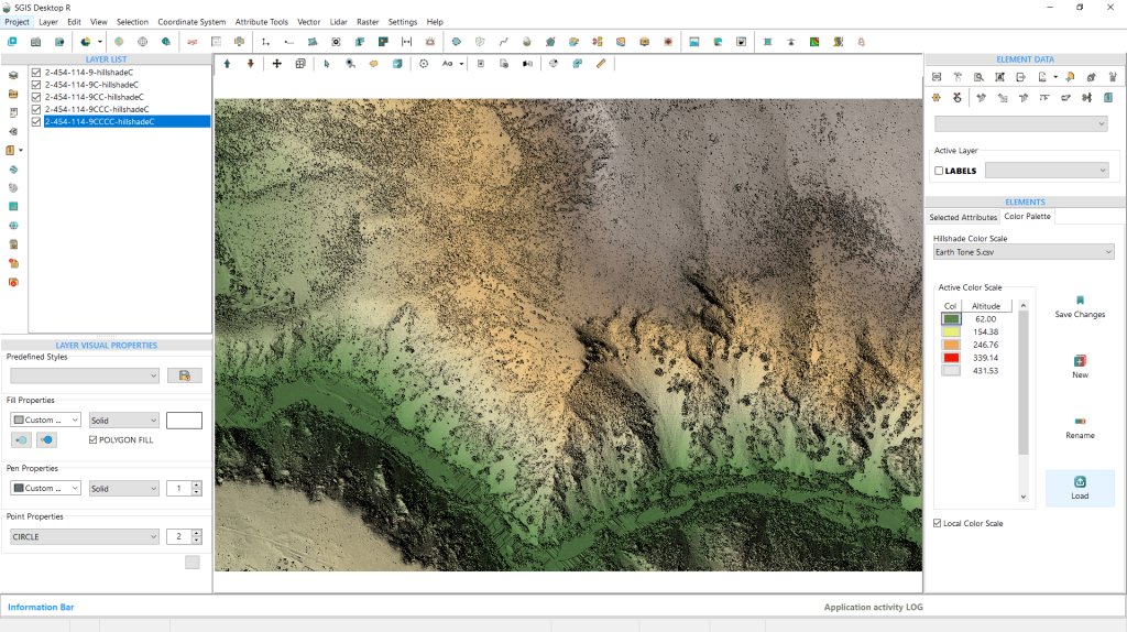
The final option is the ‘Load’ feature, which allows users to import a predefined text file containing their own color settings. The file should follow this format: ‘elevation value;R;G;B’, with semicolons separating each value. This means the file will have four columns, and users can define the number of rows, with each row representing a specific elevation value.
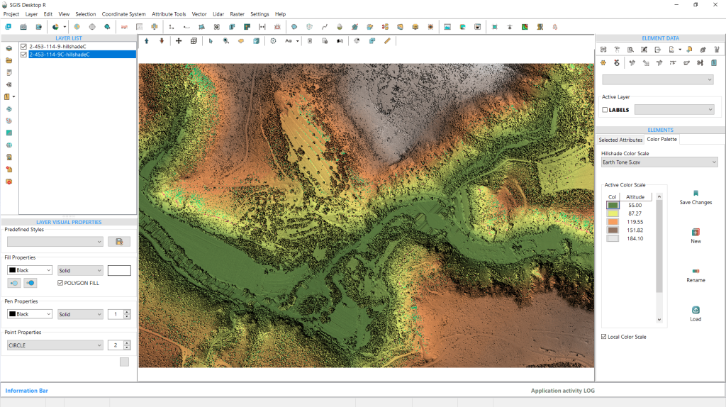
To wrap up our procedure, we’ll demonstrate the updated color scale that we previously modified. We’ve created another color hillshade DEM based on these settings. Now, we’ll switch the colors back to more subtle tones and save them once again.
This color hillshade DEM can later be exported in various formats, including DEM TIFF, Raster TIFF, JPG, PNG, or other available georeferenced raster formats.
With this, we have completed our procedure.