For this spatial join operation, you need two point layers. When the user adds these layers, SGIS automatically identifies the available spatial join relationships between them. One option provided by SGIS is ‘Points Match,’ which detects points that overlap exactly in space.
To provide a clearer understanding, let’s walk through a practical example with a telecommunications network. With our data already loaded into SGIS Desktop v1.3.1, we’re ready to move into the spatial join process. However, before we dive in, there are a few preliminary steps to cover to ensure the process is explained clearly. We’ll go through each step without skipping, showing the dataset as it currently stands and detailing all the necessary actions along the way.
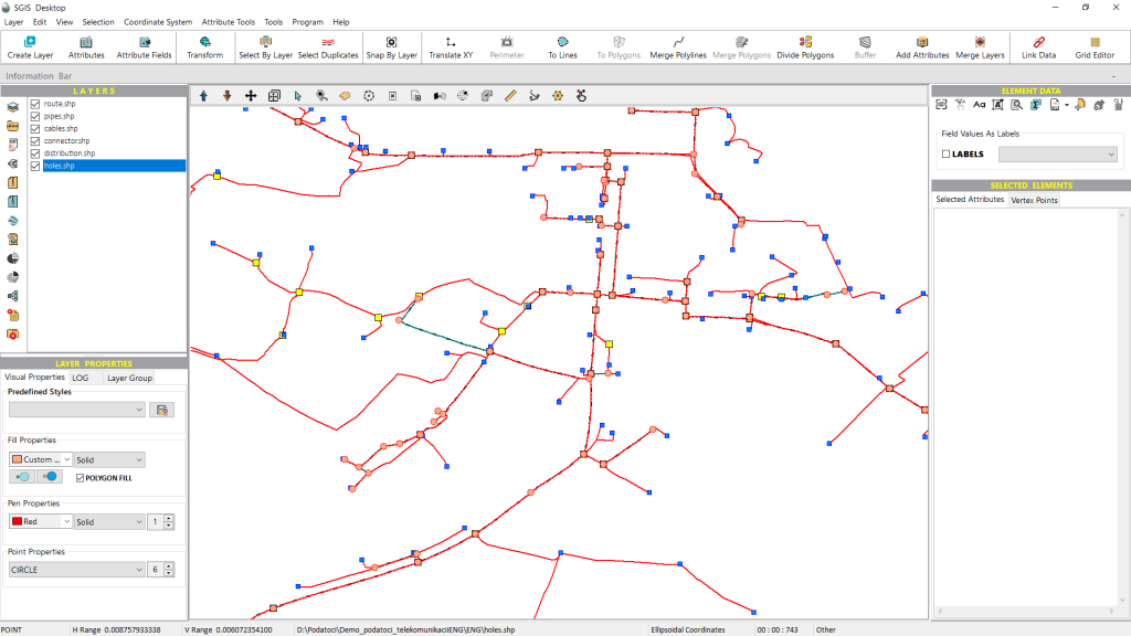
The dataset includes several SHP layers, such as telecommunication optical cables, pipelines, trench lines, connectors, telecom manholes, and distribution cabinets. As is typical in fiber optic telecommunications networks, the installation follows specific industry standards, with maintenance also governed by strict guidelines.
In these networks, it’s common practice for connector elements—like splices, splitters, and other joint enclosures—to be housed within underground telecom manholes. These manholes help protect delicate fiber optic connectors from environmental exposure and physical damage, while also providing technicians with easy access for maintenance, repairs, and future upgrades. This setup keeps network components well-organized and secure.
Each telecom manhole includes an ID field in its attribute data, which consists of a unique array of numbers identifying the network owner. Additional details, such as the manhole’s location, status, and depth, are also recorded in the attributes. This data can be linked either through ID attribute joins, or directly by the ID code itself, depending on the preferences of the provider and network owner.
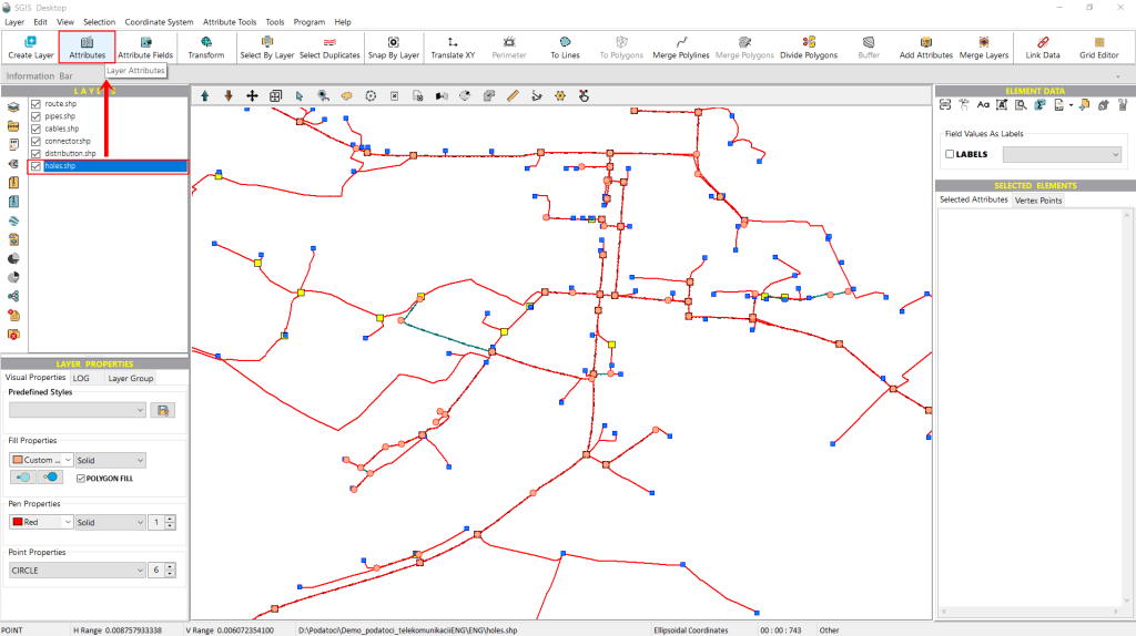
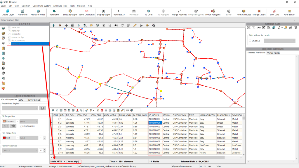
In this practical example, we’ll link the attributes from the ID_Holes field with those of the connector elements. Our goal is to ensure that each connector element has relevant data in its own attribute table, so that when an operator opens it—whether for maintenance or other purposes—they can easily identify which connector is linked to each telecom manhole. This setup will also provide details about the network owner, the location of the manhole, and other important information.
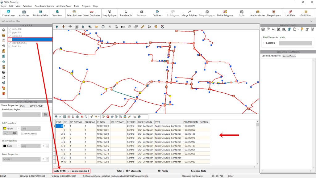
Now, let’s open the attribute table of the ‘connector’ layer. As shown in Fig. 4, there are several attribute fields within this table. To demonstrate the procedure in SGIS Desktop, we’ll first close the table to create a new field, which we’ll fill in later.
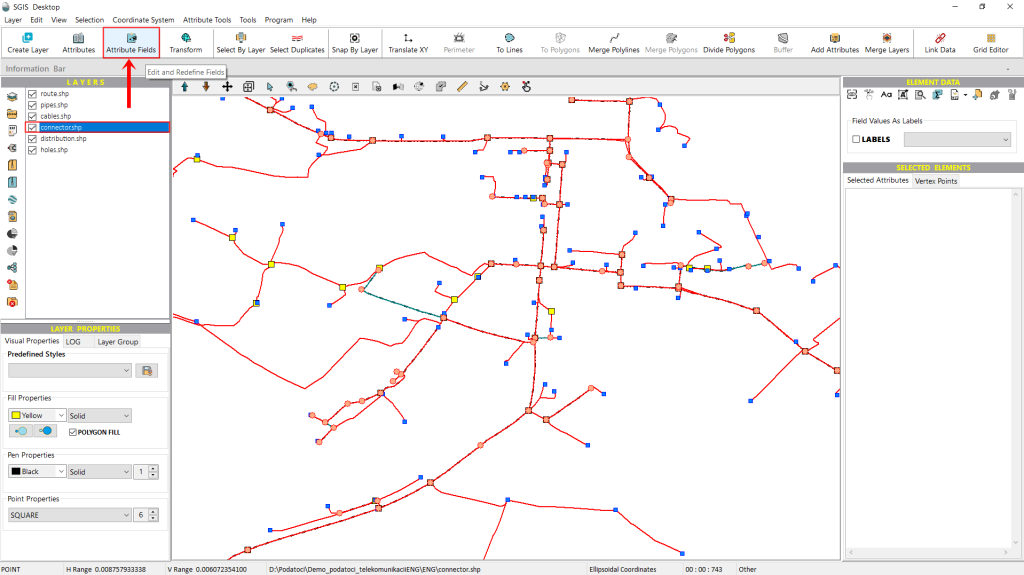
To begin, we’ll navigate to the ‘Attribute Fields’ function, conveniently located on the main toolbar. From there, we simply click to proceed.
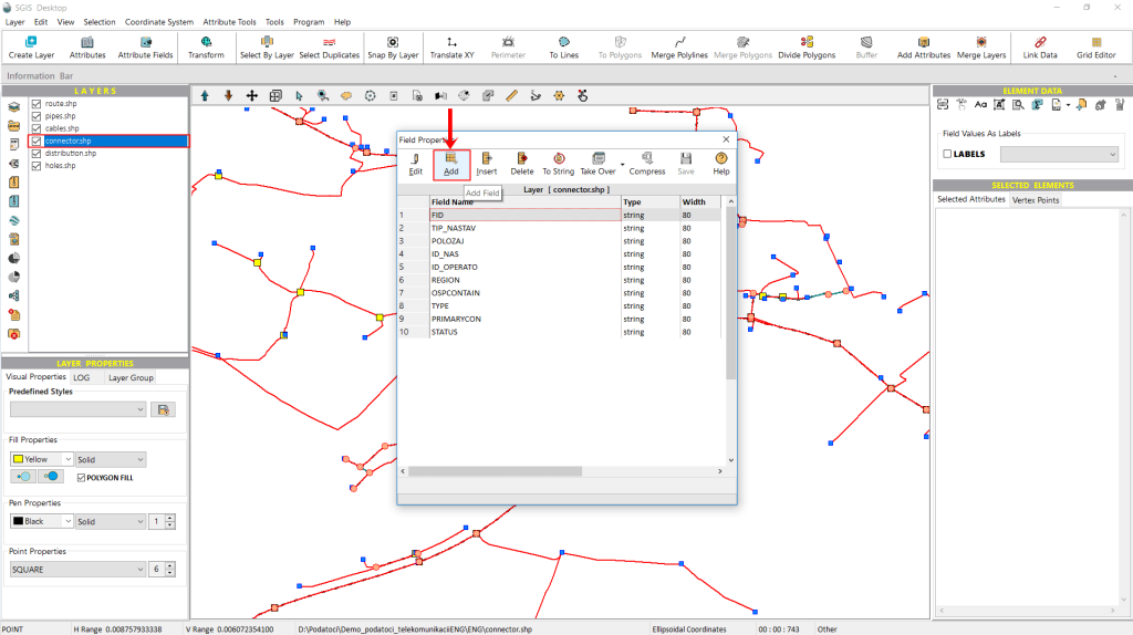
In this example, we’ll be adding a new field. Once we click on the ‘Attribute Fields’ function, a dialog window opens with various options for editing the attribute fields and structure of the attribute table. For this demonstration, we’ll focus on the specific option we need right now, while the other functions will be covered in detail in additional case studies.
Here, we simply select the ‘Add Field’ option to proceed.
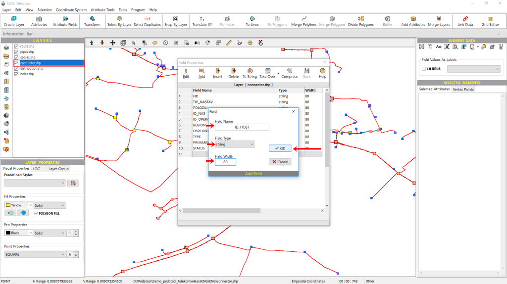
As shown in Fig. 7, after clicking ‘Add Field,’ a new pop-up window appears, prompting us to enter a ‘Field Name,’ select a ‘Field Type,’ and set the ‘Field Width.’ For this example, we’ll name the new field ‘ID_Host,’ choose ‘string’ as the field type, and set the width to 80 characters.
Next, we click ‘OK’ to confirm.
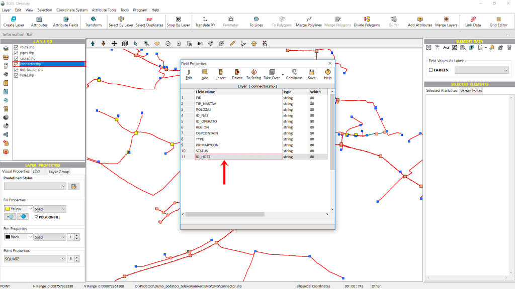
As shown in Fig. 8, the newly created field now appears in the list of attribute fields.
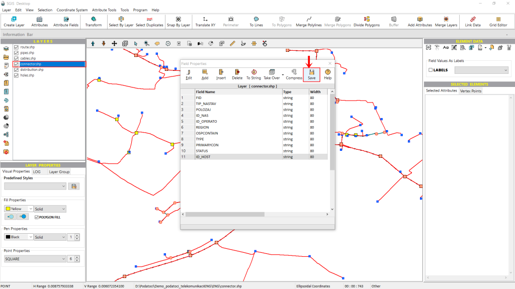
We won’t make any further changes; we just need to click ‘Save’ to apply the changes to the attribute table.
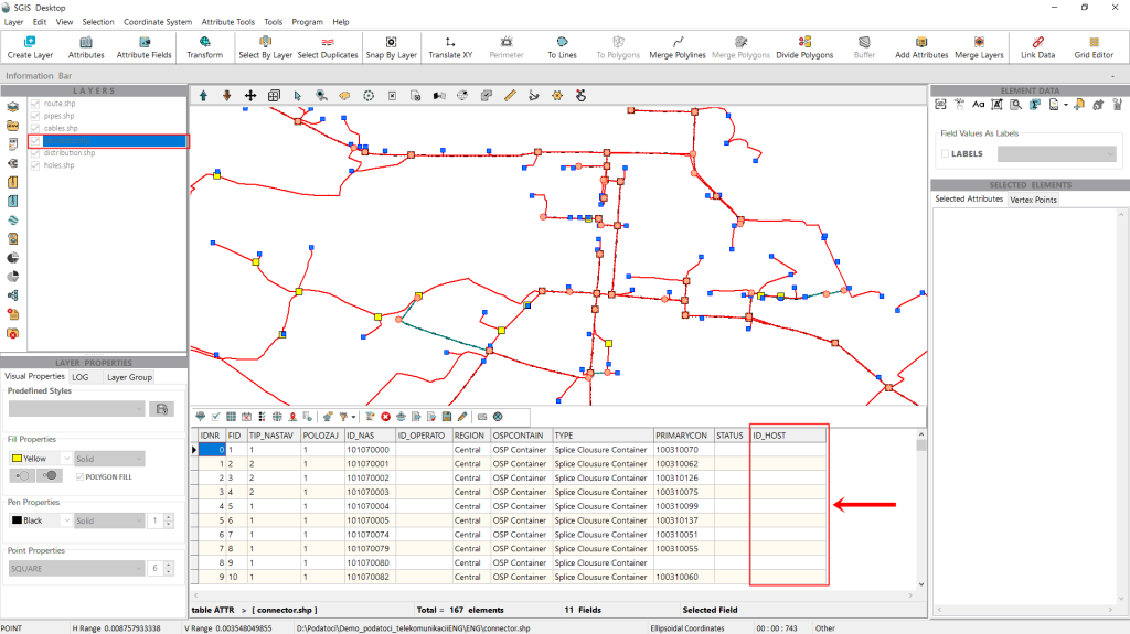
We can open the attribute table of the ‘Connector’ layer to confirm that our new attribute field has been added. As shown in Fig. 10, the field appears as expected and, since we set it to a string type, it is currently displayed empty.
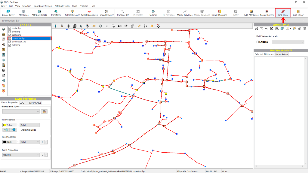
With this step completed, we can now move on to the spatial join tool, called ‘Link Data’ in SGIS Desktop and SGIS v.R. While we could have skipped creating a new field and gone directly to the ‘Link Data’ tool, using an existing field from the attribute table, this approach keeps the data more organized and clear. It also demonstrates to users without a pre-built field how straightforward it is to create one when needed.
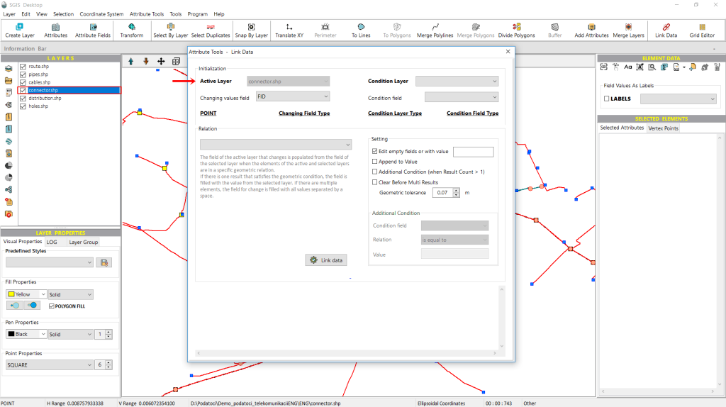
When we click on the ‘Link Data’ tool, a new window opens where we configure the necessary settings for the procedure.
Under the ‘Initialization’ tab, the first option displayed is the ‘Active Layer,’ which indicates the layer where the attribute field will be populated or modified.
The ‘Active Layer’ dropdown menu appears populated but is inactive, as the layer selection is made directly from the Layers panel. In this example, the ‘Connector’ layer is shown in the dropdown because it has been selected from the layer list.
Another useful feature in SGIS is that, upon opening the spatial join tool, it displays the type of layer selected. In bold text, it indicates that this layer is of the point type. While this may seem straightforward, it’s invaluable when working with a large number of layers in the Layers panel.
Another useful detail displayed beside the layer type is the field type selected for modification. This feature serves as a helpful reminder, especially when ensuring that we’re working with the correct field type. For instance, we may have created a string field when an integer was needed, or an integer when a double would be more appropriate. Having this information readily available saves time by preventing unnecessary steps later in the process.
Additionally, SGIS displays both the field type of the attribute table in the active layer (which will be modified) and the field type of the condition layer (from which we will pull data). This clarity aids in ensuring compatibility between fields in the spatial join process.
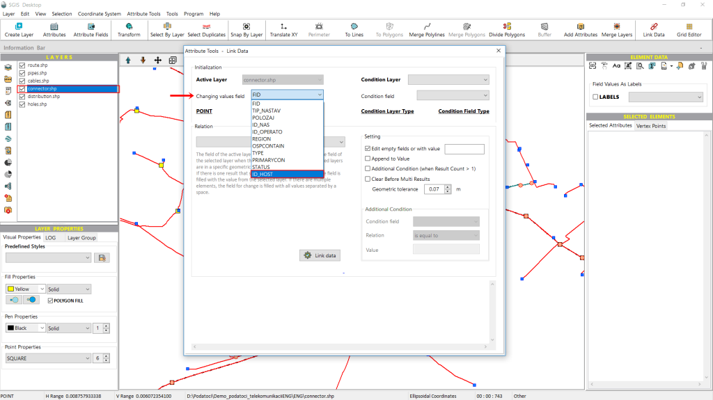
Next, we need to select the field that will be updated with new values. To do this, we open the dropdown list and choose the field we previously created for this example, named ‘ID_Host’.
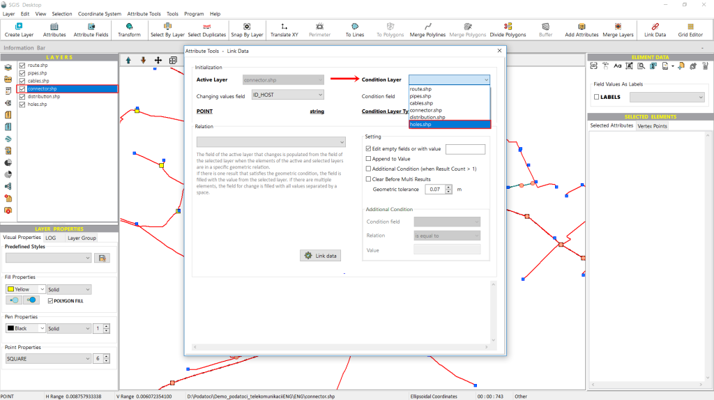
After selecting the field to be updated, we complete the settings for the ‘Active Layer’ on the left side of the window. Now, we need to configure the settings for the ‘Condition Layer.’
To do this, we open the dropdown list and choose which layer from the Layers panel will serve as the condition layer. Unlike the previous dropdown, this one is enabled, allowing us to pick the layer with the required attribute field. In this example, we select the ‘Holes’ layer, as it contains the ‘ID_Holes’ attribute field we need.
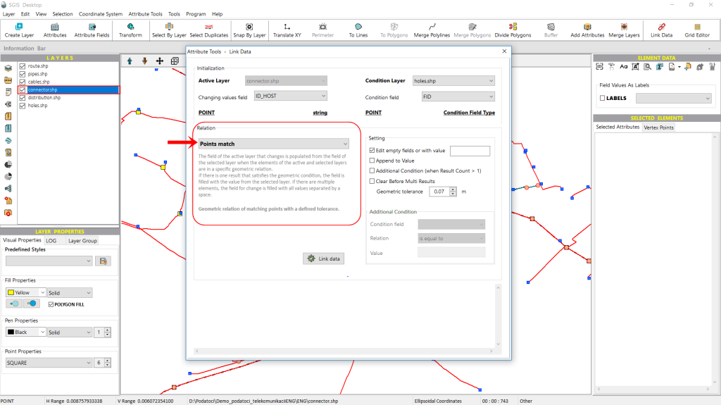
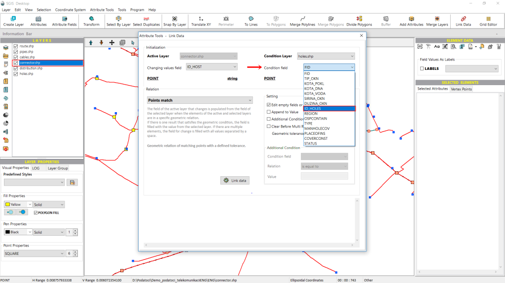
In the ‘Relation’ tab, just below the displayed ‘Points Match’ spatial join relationship, there is a memo box explaining how the relationship functions.
It states that the field in the active layer, which will be updated, will draw its values from the selected field in the condition layer whenever elements in both layers share the specified geometric relationship. If a single match meets the geometric condition, the field is populated with that value from the condition layer. If multiple elements satisfy the condition, all matching values will be included in the updated field, separated by spaces.
Additionally, this geometric relationship can be adjusted with a user-defined tolerance.
On the right side of the ‘Relation’ tab, there is another tab called ‘Settings’ that provides additional configuration options. Let’s go through them individually.
The first option is a checkbox labeled ‘Edit empty fields or with value ___’. When selected, this option allows the procedure to populate only the empty fields in the attribute column. If we enter a specific value, only the fields that already contain that value will be updated.
The second option is the ‘Append to Value’ checkbox. When selected, this allows the procedure to update attribute fields that already have values by adding the new data to the existing values, rather than replacing them.
Next is the ‘Additional Condition’ checkbox. When enabled, it activates new input fields where users can define custom conditions and specify their desired values.
The next option is ‘Clear Before Multi Result,’ which allows users to clear the field when multiple results are present.
The final option is ‘Geometric Tolerance,’ which users can adjust to suit their specific requirements.
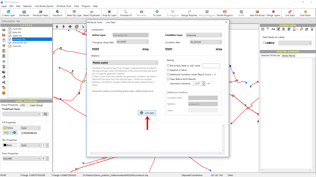
After configuring all the desired settings and clicking on ‘Link Data,’ the software will display a confirmation message once the process is complete.
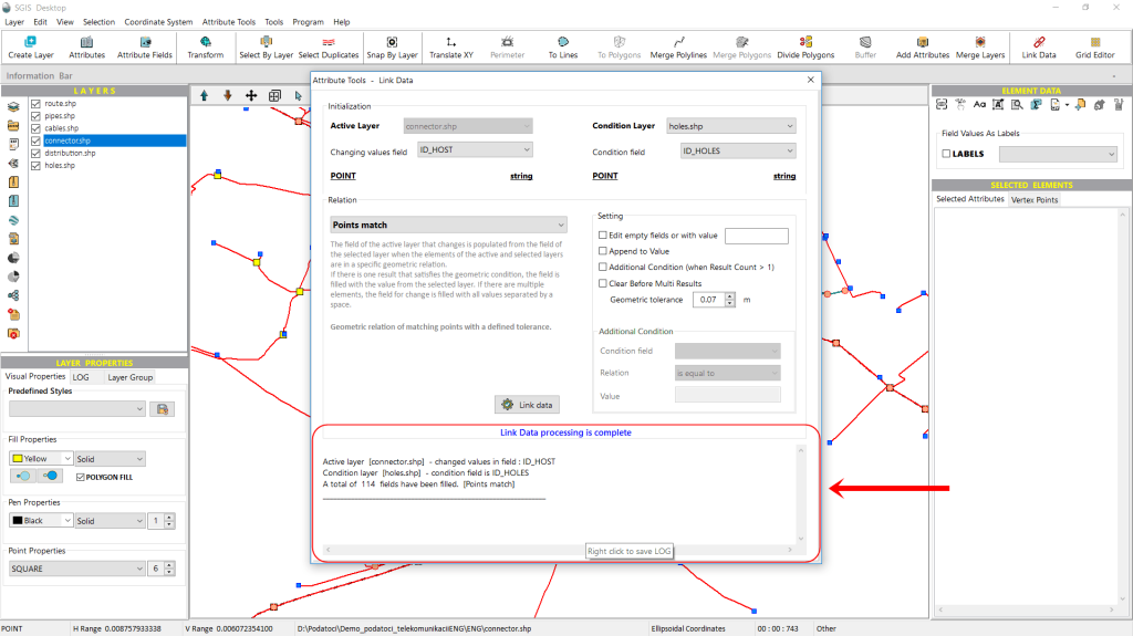
In the memo box at the bottom of the ‘Link Data’ dialog window, SGIS provides a detailed summary of the operation. It specifies the Active Layer (in our example, the Connector layer), the attribute field populated (in this case, ID_Host), the Condition Layer (the Holes layer in our example), and the condition field from which the data was taken (ID_Holes).
Additionally, it reports how many elements satisfied the geometric condition ‘Points Match,’ indicating the total number of modified or populated fields.
For record-keeping or troubleshooting, this information can be saved as a LOG file by right-clicking on the memo box.
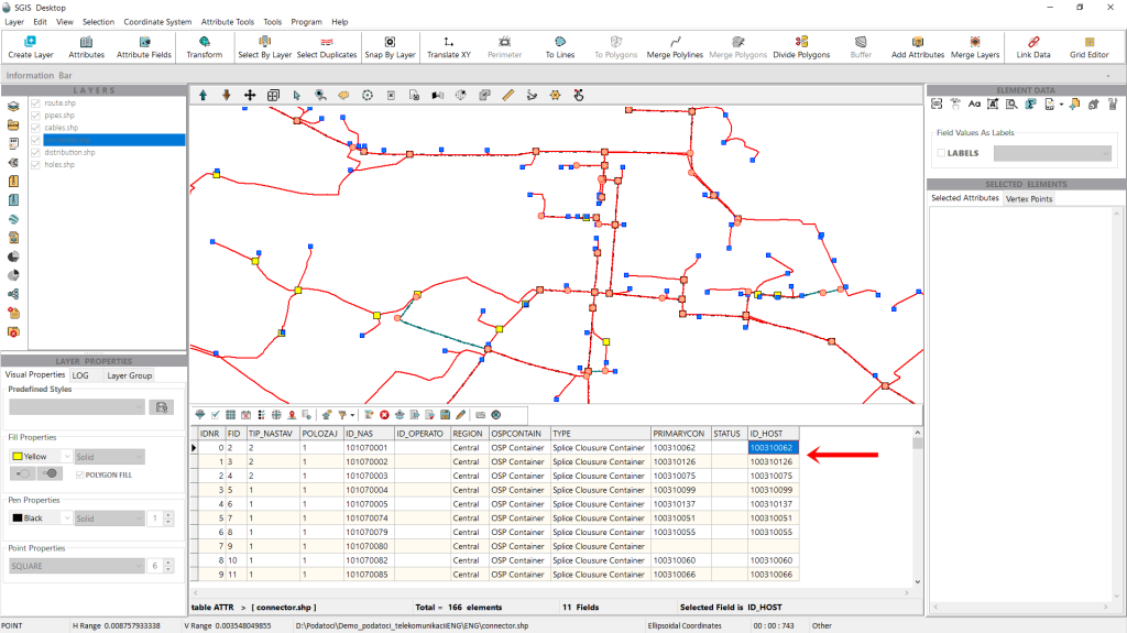
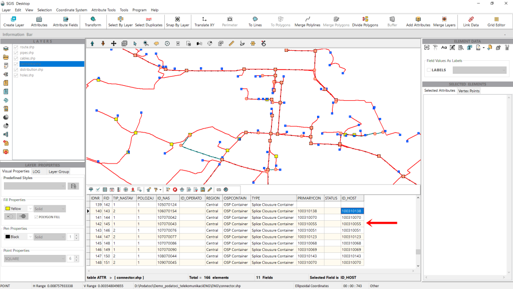
After completing the procedure, we can open the attribute table of the Connector layer to review the results.
As shown in Fig.19 and Fig.20, the ID_Host field has been successfully populated with the corresponding values.
With this, the procedure is complete!