SGIS v.R Technology: Developing an Improved Algorithm
Developing Enhanced Algorithm for GIS Software Environment to Achieve Millimeter-Level Coordinate Transformation Accuracy
Published on: 29.07.2024
Integrating various sets of geodetic data into a single, consistent dataset within a common geodetic reference frame is crucial when handling geospatial data. This becomes evident as soon as one starts using GIS. The core of GIS lies in having multiple data layers that overlap accurately, which is only possible if they are precisely positioned and correctly georeferenced.
Transforming data from one reference frame to another involves applying a coordinate transformation. While the math behind these transformations is straightforward, practical issues can, and often do arise.
SGIS v.R Technology
Validating Algorithm Precision with Forward-Inverse Coordinate Transformations Using Real GIS Data
To verify the precision and accuracy of our algorithm, we will compare the original coordinates with those obtained after performing forward and inverse transformations. This method is rooted in mathematical principles and practices, commonly used in fields like geodesy, computer science and numerical analysis.
In mathematics, an inverse function essentially “undoes” the action of the original function. For coordinate transformations, verifying the process by using the inverse function tests whether the transformation and its inverse are implemented correctly. This practical application of inverse functions ensures that the theoretical properties of these mathematical constructs are preserved in the computational algorithms.
Essentially, this means that the forward and inverse transformation represents a bijective function pair, meaning each coordinate in the original system has a unique counterpart in the transformed system and vice versa. By ensuring that applying the forward transformation followed by the inverse transformation returns the original coordinates, we confirm the correctness and consistency of the transformation functions. This is akin to proving that the functions are reversible, which is a fundamental property in mathematical analysis.
What is important for us is that round-trip transformation (applying forward and then inverse transformation), detects numerical errors and assess the precision of the transformation algorithms. Numerical computations, especially those involving floating-point arithmetic, can introduce small errors.
By verifying that the original coordinates are recovered after the inverse transformation, we ensure that these errors are within acceptable limits, maintaining the precision required for high-accuracy applications.
In numerical methods and computer science, stability refers to an algorithm’s ability to produce accurate results despite small perturbations or rounding errors. Verifying coordinate transformations through round-trip consistency checks demonstrates the stability and robustness of the transformation algorithms. This is particularly important in geospatial applications where small errors can propagate and amplify through subsequent computations.
To begin, we have a dataset of polylines representing underground telecommunications pipelines. We start by loading the shapefile into SGIS v.R. To better understand the location, we’ll add a Tile Map Service in the background, using OpenStreetMap as an overlay. The real-time coordinates are displayed in the bottom-right corner, showing that the data is saved in the WGS 84 coordinate system.
Fig. 1 Data loaded into SGIS v.R with a basemap for enhanced understanding.
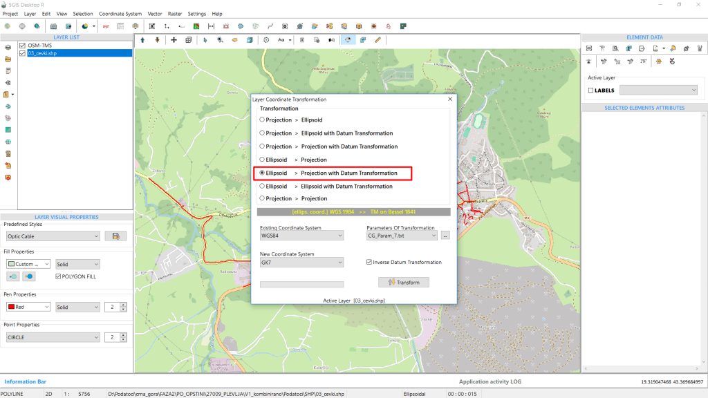
First, we need to access the ‘Layer Coordinate Transformation’ function, which can be found in the Coordinate Transformation menu on the main Menu Ribbon. The user is prompted to select the existing coordinate system from the dropdown list, where we’ll choose WGS84.
Fig. 2 Selected Transformation - Ellipsoid to Projection with Datum Transformation
Next, the user selects the desired coordinate system for the transformation. In this example, we’ll select the preset GK7, an alias for Gauss-Kruger zone 7 (MGI Balkans zone 7).
The ‘Transformation’ upper menu, which defaults to ‘Ellipsoid to Projection with Datum transformation,’ is auto-selected once the existing and desired reference frames are chosen. This indicates that our transformation is a Datum ellipsoid to projection coordinate transformation.
After selecting the transformation parameters from the dropdown list, we click ‘Transform’.
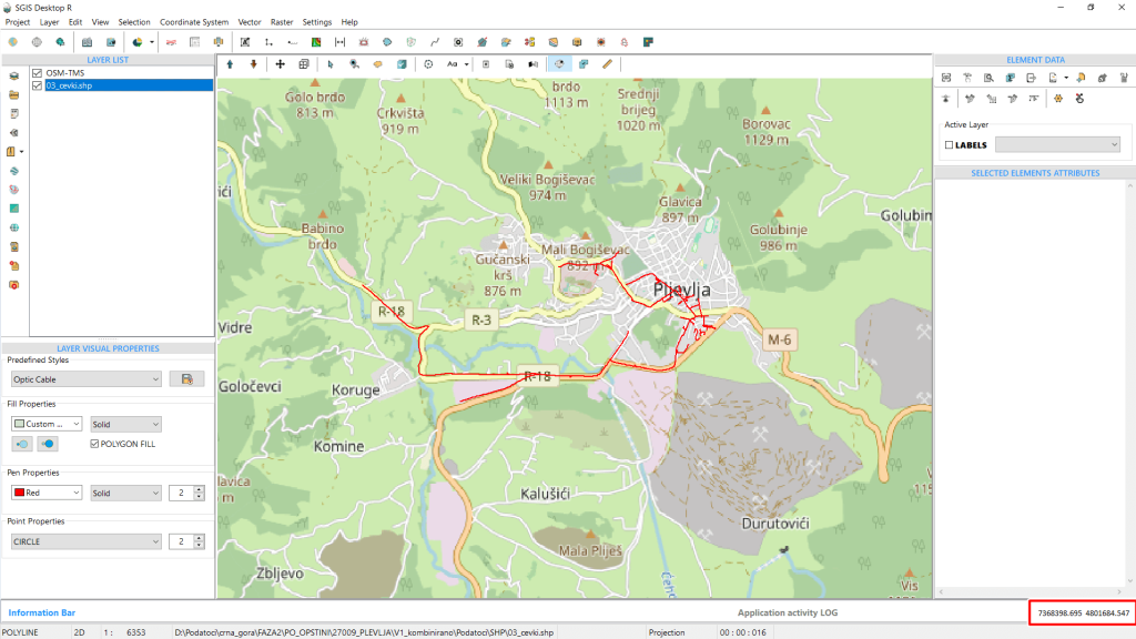
Fig. 3 The transformation process completed, showing the coordinates of the extent in the bottom-right corner
The completion of the transformation is immediately visible in the bottom-right corner where the coordinates are displayed.
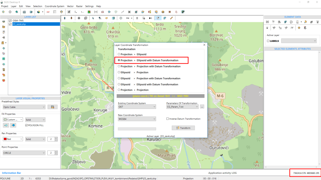
The layer is transformed ‘on the fly,’ and no new layer is created in the Layers panel. Next, we’ll proceed with the inverse transformation by converting this layer back to WGS84.
Fig. 4 Initiating the Inverse Coordinate Transformation from Gauss-Kruger to WGS84
To compare the results, we add the transformed layer to the list of layers and load the original file. Both shapefiles are in WGS84.
Fig. 5 Original and Transformed Layers Loaded in the Layers Panel for Visual Coordinate Comparison
We can visually compare the coordinates from both layers by examining their overlay in the graphics window. When zooming in, the overlap is exact, with the lines perfectly aligned. For better visual clarity, one layer is displayed as a solid red line, while the other is shown as a lime green dashed line.
Fig. 6 Close-up View Comparing Coordinate Overlays Between Layers, Demonstrating Perfect Line Alignment
To complete the process, we’ll select a segment of the lines representing the pipelines and export its coordinates from both the original and the converted layers.
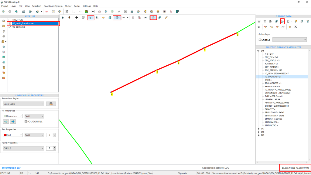
Fig. 7 Segment Selected for Exporting Coordinate Vertices
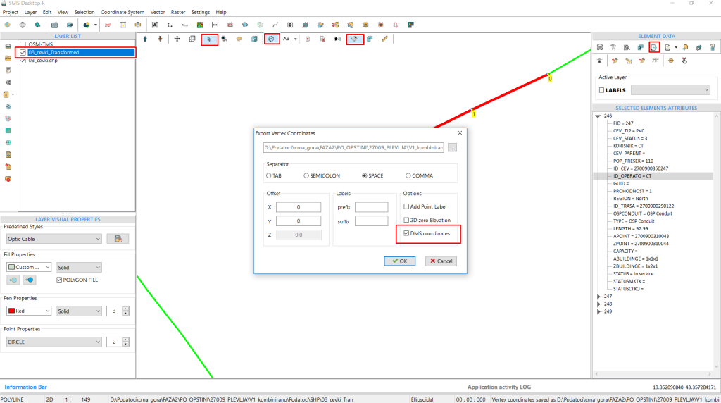
To do this, we need to select the layer from the Layers Panel and activate the Selection and Vertex functions. Left-click on the desired line to select it, then choose “Export Vertex Coordinate” from the element data toolbox.
The “Export Vertex Coordinate” function will open a dialog window where the user can set preferences such as the save path, separator, offset, and other options. In this case, we’ll check the box for ‘DMS coordinates’ to export the coordinates in Degree Minutes Seconds format. Finally, click OK.
Fig. 8 In the Export Vertex Coordinate Dialog Window, Check the Box for DMS Coordinates to Export Vertices in Degrees Minutes Seconds Format
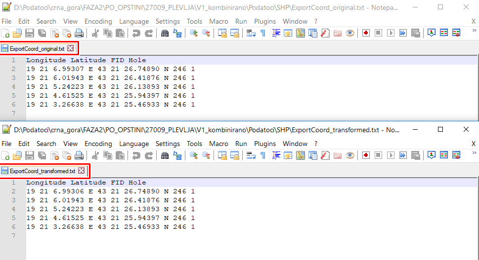
For the final comparison of the coordinates, we opened both files previously exported as text files with DMS coordinates from the original and transformed shapefiles. The files consist of four columns: Longitude, Latitude, FID field, and Hole. Comparing the first row in the longitude column, we see that the value differs by only 0.00001 seconds, while all other values are exactly the same.
Fig. 9 Final Comparison of Coordinates Opened as DMS Coordinates in Separate Text Files
This confirms the accuracy of the transformation process in SGIS v.R technology.