LIDAR Project Processing: Opening and Managing Multiple LAS Files by Defining Project Boundaries
Published on: 30.09.2024
Handling large-scale LIDAR datasets, like multiple LAS files, can be a challenge. By defining project boundaries, users can focus on loading only the relevant data, making the process more efficient and cutting down on unnecessary processing. This approach prevents systems from becoming overwhelmed when dealing with large datasets, as it minimizes memory usage and computational strain. By working with smaller, more targeted sections of data, users can avoid slowdowns and boost processing speed, ensuring a smoother workflow overall.
SGIS v.R offers this feature through its ‘View LiDAR Boundaries’ tool. With this tool, users can easily select the number of LIDAR files they need, and it will automatically display the boundaries of all the selected files on the graphics panel. From there, users can quickly open any LAS file within the desired boundary for further analysis, making it a highly efficient way to manage and visualize large LIDAR datasets.
To illustrate how this function works, we’ll walk through a practical example by loading several LAS files into the software. This will give users a clear idea of how the tool operates and how easily multiple files can be opened and managed within the project.
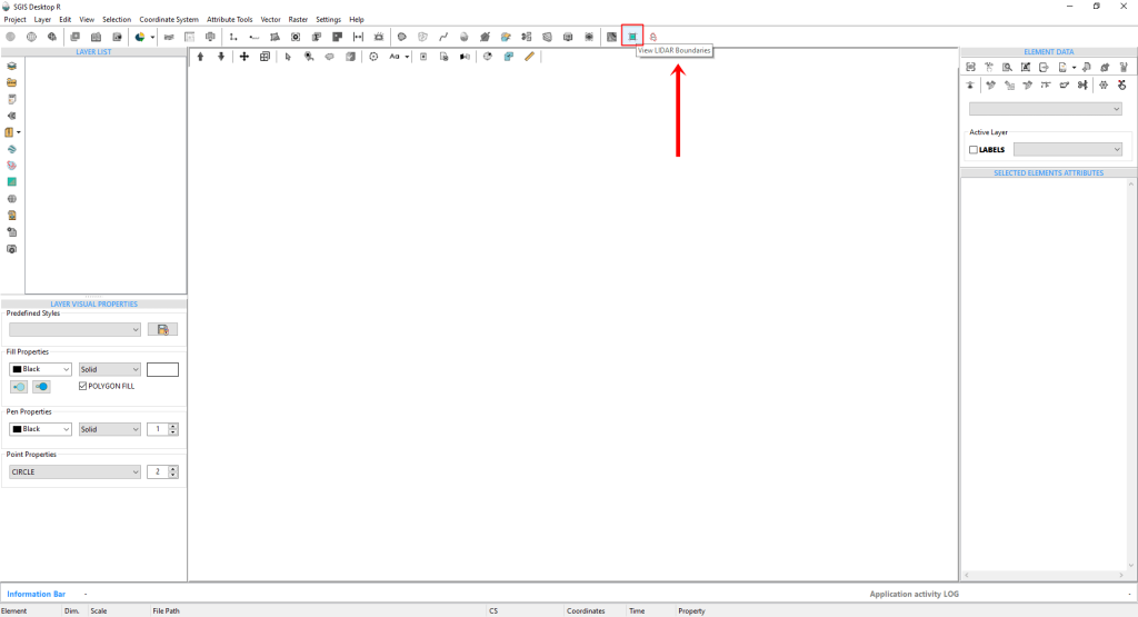
Fig.1 The ‘View LiDAR Boundaries’ tool, accessible from both the Project menu and the main toolbar in the user interface.
To get started, simply click on the tool.
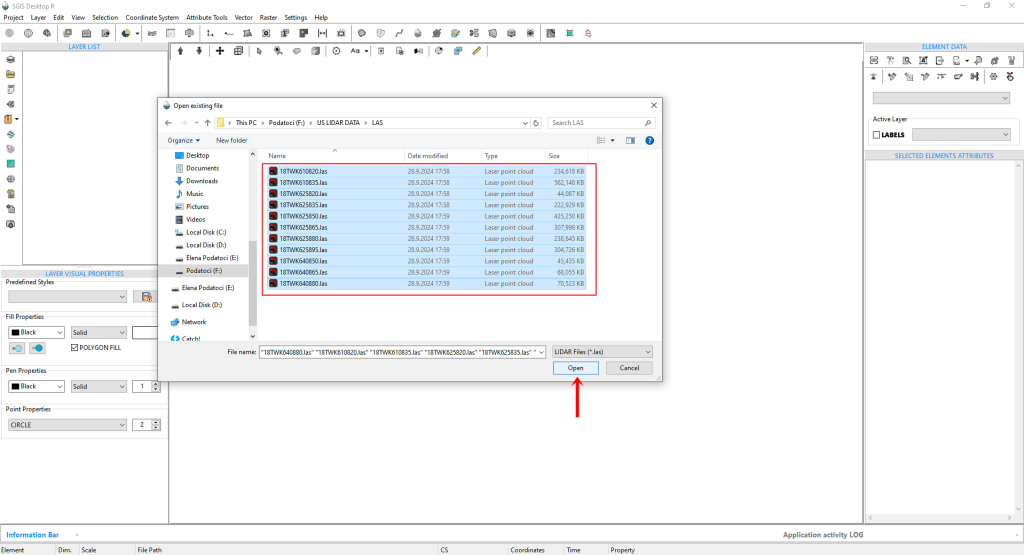
This will bring up an ‘Open File’ dialog box where you’ll need to navigate to the folder containing your LAS files. Once you’ve located the folder, you can easily select all the LAS files by clicking on one and then pressing CTRL+A.
All the files should now be highlighted and ready for the next steps.
Fig.2 The ‘Open File’ dialog box appears after clicking the tool, prompting users to navigate to the folder with their LAS files.
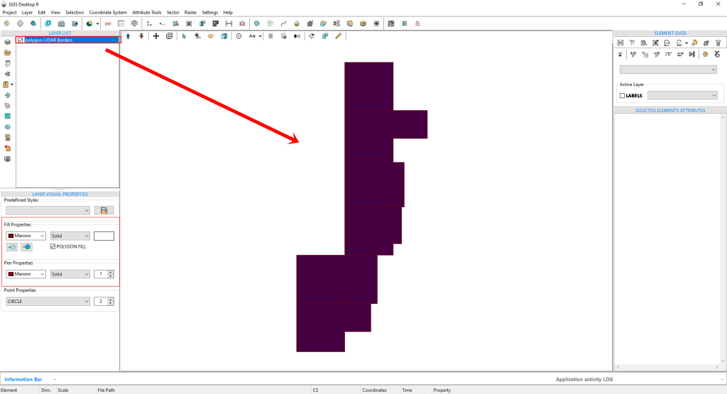
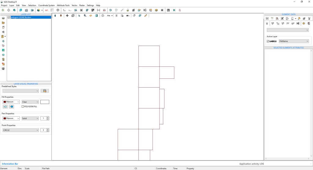
After clicking ‘Open,’ the LIDAR boundary polygons will quickly appear on the Graphics panel. Initially, these polygons will be filled with a random color. However, users have the option to customize the appearance by adjusting the pen and fill colors to their preference.
Fig. 3 After clicking ‘Open,’ the LIDAR boundary polygons will quickly appear on the Graphics panel.
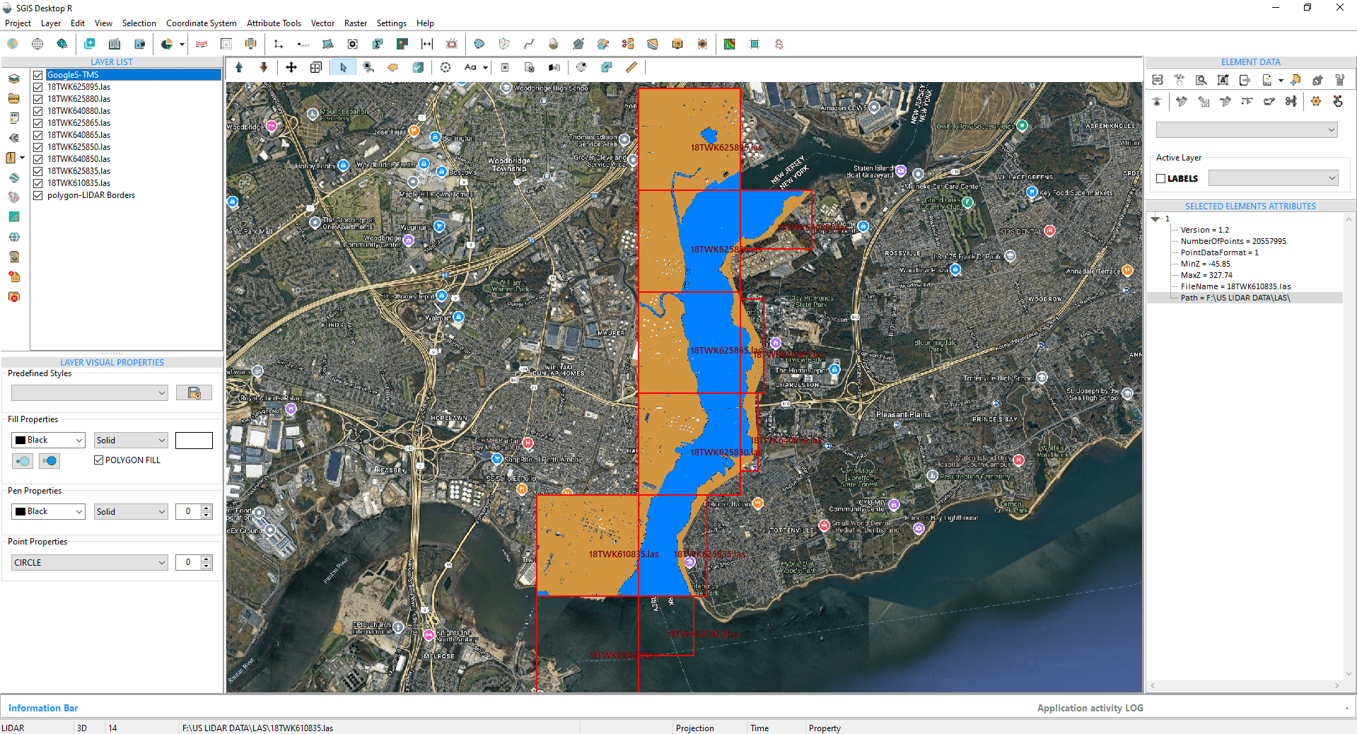
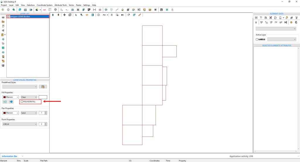
Fig.4 The ‘Polygon FILL’ option is unchecked to eliminate the fill color within the polygon areas. This change enhances visibility and clarity for users as they prepare to import the LIDAR point cloud within these defined boundaries.
We’ll uncheck the ‘Polygon FILL’ option to remove the fill color inside the polygon areas. This adjustment will make it easier to work with as we import the LIDAR point cloud within these boundaries.
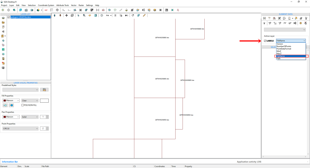
Fig.5 To enhance our workflow, we activated the labels and selected the ‘FileName’ field from the dropdown menu. This adjustment displays the file name on each polygon, offering users a clearer visual reference.
To streamline our workflow, we’ll activate the labels and choose the ‘FileName’ field from the dropdown menu. This will display the file name on top of each polygon, providing a clearer visual reference for users.
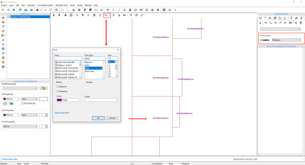
The Labels Visual Style can also be customized. By clicking on the ‘Font’ option, you can change the font type, style, size, height, color, and more. However, for the purposes of this demonstration, we’ll keep the current settings as they are.
Fig.6 The Labels Visual Style can be customized further. By clicking on the ‘Font’ option, users can modify various attributes such as font type, style, size, height, and color.
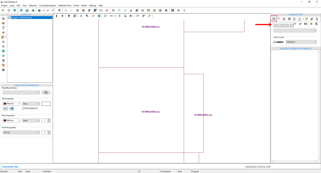
Fig.7 The 'Label Visibility Border' feature in SGIS v.R allows users to set a specific zoom level for label display on the Graphics panel. When activated, labels appear when zoomed in and disappear when zoomed out, helping to reduce clutter on the screen.
SGIS v.R offers an additional feature for managing labels on the Graphics panel called the ‘Label Visibility Border.’ This simple one-click option allows users to define a specific zoom level at which labels will be visible. When we activate this function, as shown in Fig.7, labels will appear when zoomed in and disappear when zoomed out. This helps prevent data overload on the graphics panel.
Let’s go ahead and click to activate this option.
Fig.8 After zooming out, the labels become invisible due to the activation of the 'Label Visibility Border' feature.
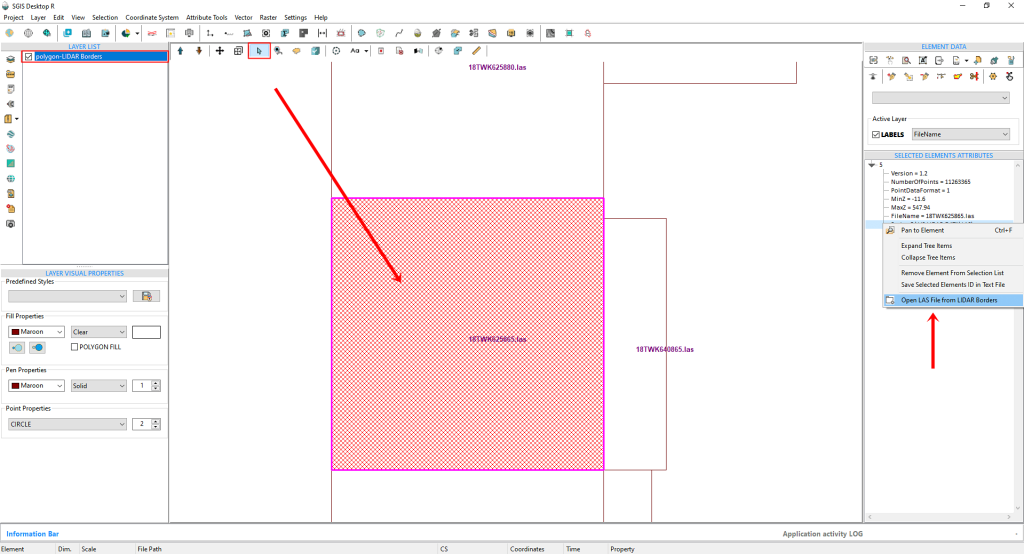
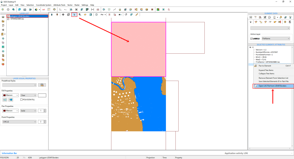
The next step in our process is to zoom in and select a specific polygon area. To do this, we simply need to activate the ‘Select’ function. By clicking on the polygon boundary, it will become highlighted, and in the ‘Selected Elements’ panel on the right side of the user interface, we can view the attributes of the selected polygon. We then click on any field displayed in the rows of the ‘Selected Elements’ panel and right-click on it. A dropdown menu will appear, where we can select ‘Open LAS file from Boundary’.
Fig.9 Loading a LAS file through the polygon boundary.
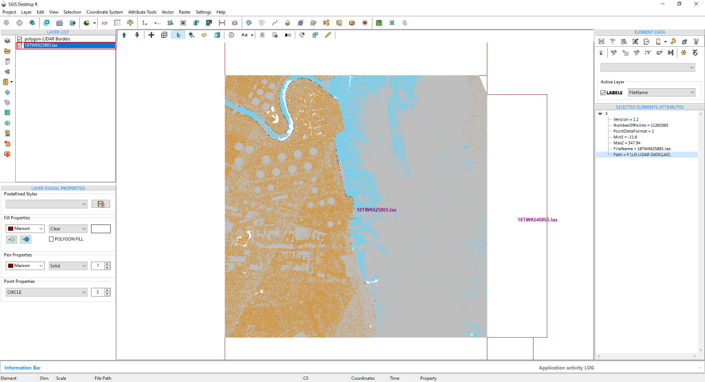
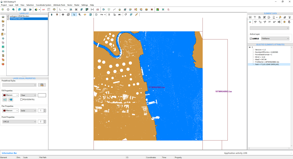
The LAS file has successfully loaded. Since it comes with predefined ASPRS classification color properties, we’ll open the LIDAR toolbox to adjust some of these settings for better visual clarity.
Fig.10 The LAS file has been successfully loaded into the software.
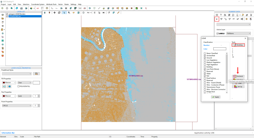
Fig.11 In the LiDAR toolbox, we first click on ‘Existing’ to view the list of current classifications. We then select ‘Uncheck’ to clear all empty boxes.
In the LiDAR toolbox, we start by clicking on ‘Existing’ to view the memo list of current classifications. Next, we select ‘Uncheck’ to deselect all empty boxes from the Classification list. For clearer visualization, we’ll also uncheck Class 1, as almost all non-ground points in this LiDAR dataset are classified as Unclassified.
Fig.12 For improved visualization, we’ll also uncheck Class 1, as all non-ground points in this dataset are classified as Unclassified.
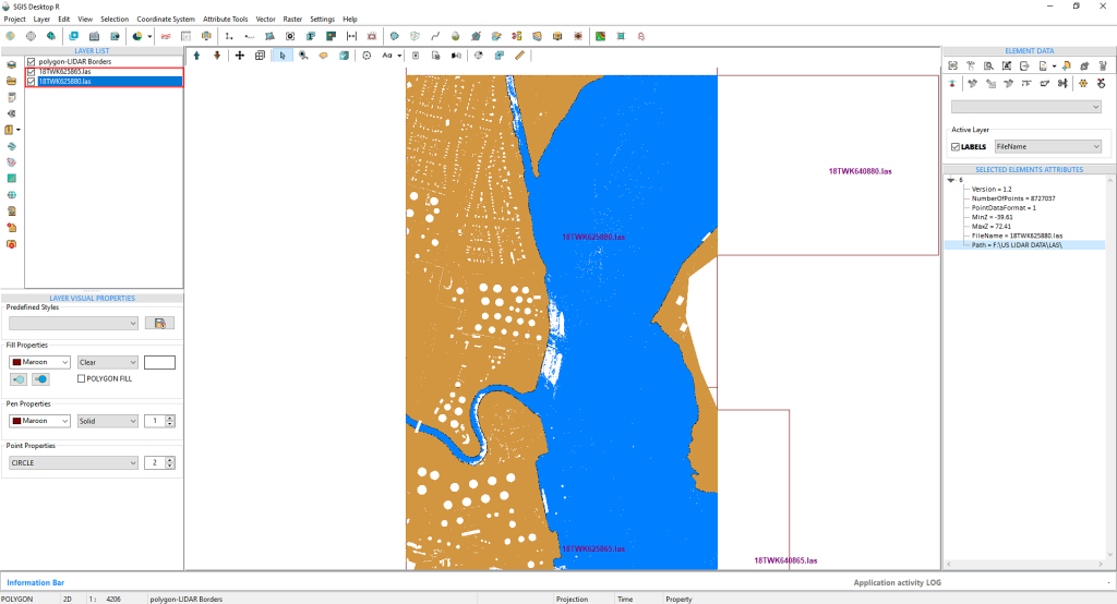
Fig.13 To open the second tile, we activate the Selection function and click inside the tile. Then, we can right-click on the ‘Selected Elements Attributes’ to access the second LAS file.
To open the second tile, we’ll activate the Selection function and simply click inside the next tile. After that, we can right-click on the ‘Selected Elements Attributes’ to open the second LAS file.
The LAS file loads instantly, retaining the visual settings we adjusted for the first file using the LiDAR toolbox.
Fig.14 The LAS file loads promptly, maintaining the visual settings we applied to the first file through the LiDAR toolbox.
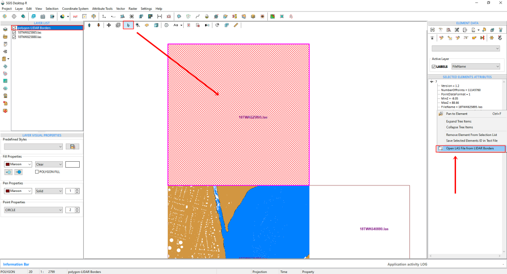
Fig.15 We will continue the same process to open the third tile and can repeat this for as many tiles as necessary.
We’ll use the same approach to open the third tile, continuing this process for as many tiles as needed.
Additionally, we can load a Tile Map basemap to get a better view of the terrain and gain more insight into the urban area, as these LAS tiles are part of a city landscape. This extra layer helps in identifying features for further analysis or reclassification. To access the Tile Basemap, simply click on ‘Tile Map Servers’.
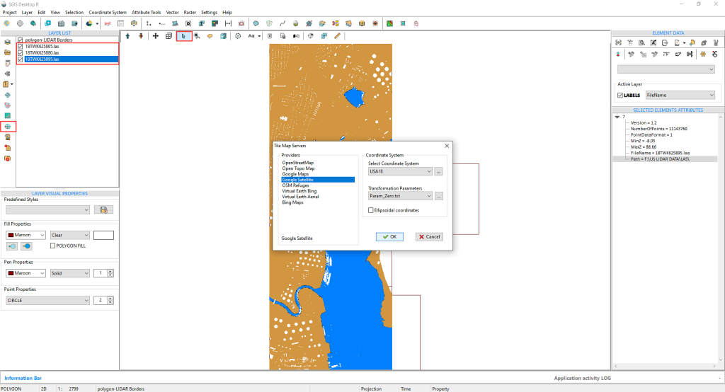
Fig.16 Selecting Google Satellite as the basemap, we choose the coordinate system and transformation parameters from the dropdown menus. The coordinate systems are predefined with EPSG codes, but users can input their custom settings and save them under an alias for future use.
We’ll select ‘Google Satellite’ and then, on the right side, choose the ‘Coordinate System’ and ‘Transformation parameters’ from two dropdown menus. The coordinate systems are predefined with their EPSG codes, but users have the option to input custom settings and save them with an alias for easier recall.
For instance, we’ve already saved our coordinate system under the alias ‘USA18’ for quick reference and convenience.
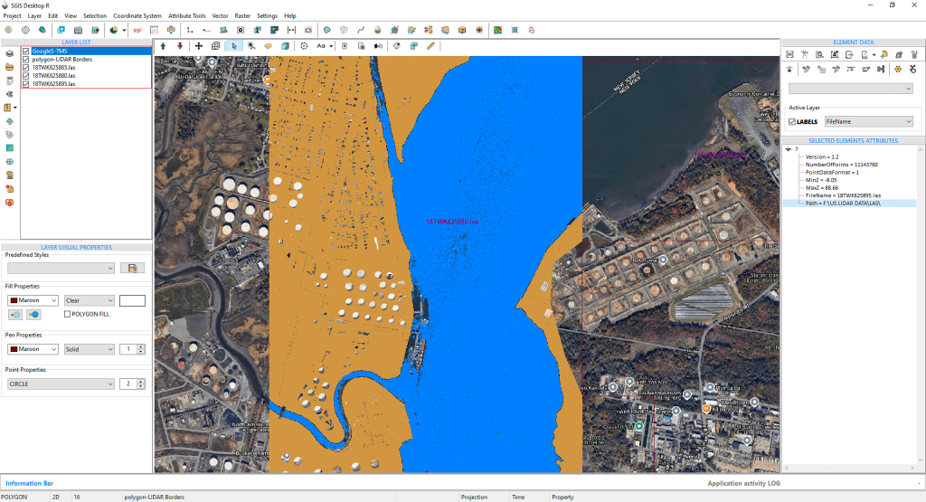
Fig.17 The Google Satellite basemap aligns accurately with the LAS tiles, ensuring precise spatial overlap for further analysis.
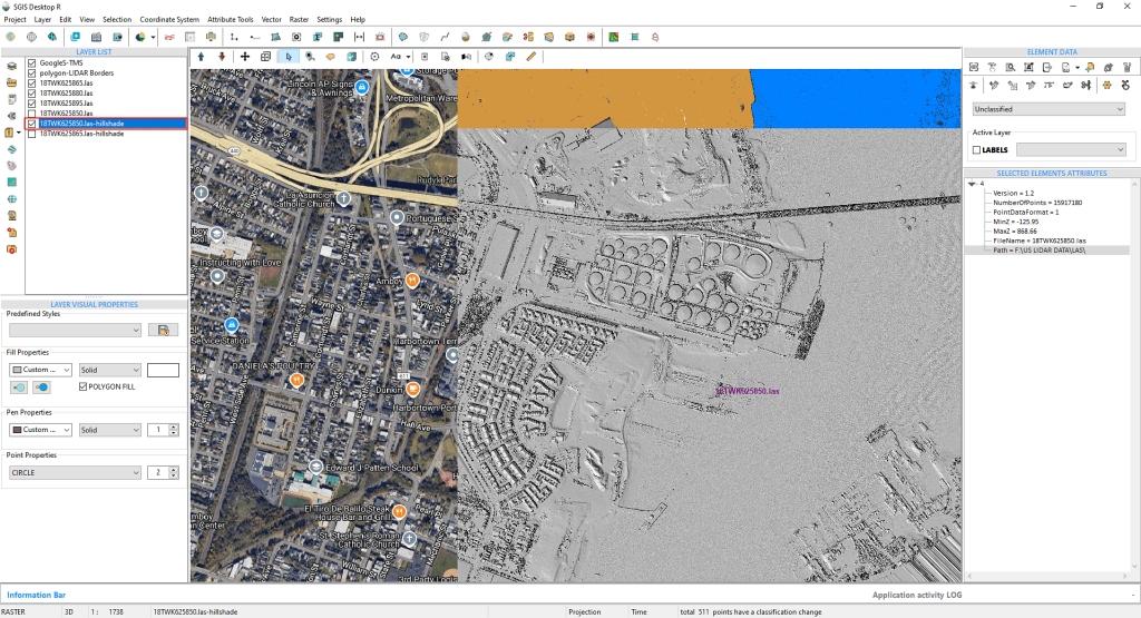
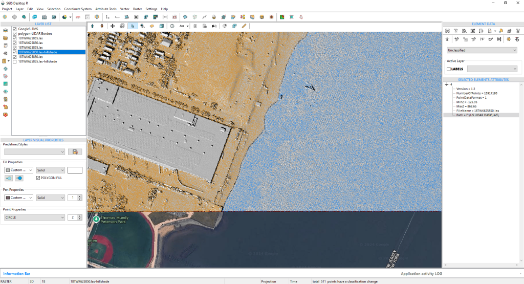
Fig.18 The hillshade layer, generated using the ‘Create Grid’ function, provides a clear 3D view of the terrain, highlighting elevation and topographic features. This is especially useful in urban areas, where it helps visualize how buildings and roads integrate with the landscape.
Users have the option to either add an existing hillshade layer or create one using the ‘Create Grid’ function. This enhances the three-dimensional visualization of the terrain, making it easier to detect elevation shifts, slopes, and subtle topographic features that may not be immediately apparent from the point cloud data. In urban environments like the one in our example, where natural and man-made structures coexist closely, a hillshade basemap helps users better visualize how features like buildings and roads interact with the surrounding landscape.