Developing an Algorithm for Direct Color Hillshade Creation from LAS (by interpolation), ASCII DEMs, and any Active DEM Layers
Published on: 07.11.2024
A color hillshade is an elevation map that blends shaded relief with color gradients, providing a vivid depiction of terrain. By combining shadows and colors, it enhances the perception of depth and reveals intricate details of topographic features.
By ‘Direct Color Hillshade Creation,’ we mean an efficient way to generate colorized hillshade DEMs directly from a LAS file (by interpolating point data), from an ASCII DEM (Digital Elevation Model) file, or any active GIS layer with elevation data (such as DEMs, for e.g., in TIFF format), without requiring extra steps like file conversion or multiple styling processes.
In most GIS software environments, creating a color hillshade typically involves several stages and requires multiple layers (at least two). Users generally open the DEM, apply color ramps (often using single-band pseudocolor options), create a separate hillshade layer, and then blend the two layers to achieve the final effect. While effective, this process can be time-consuming, complex, and not very straightforward.
With SGIS, we’ve simplified the process to make it much easier for users. We’ve made it possible for users to open a LAS file and directly interpolate a color hillshade DEM, or load an ASCII DEM, select an elevation-based color ramp, and let SGIS automatically generate the colorized hillshade DEM, which can then be exported as a DEM or a raster image file (georeferenced raster image file). There’s no need for multiple styling steps or blending modes—just one step, and the color hillshade is ready.
We’ve made this available through several loading options, and we’ll demonstrate some of them with practical examples.
Enhancing Terrain with Color
Color gradient (elevation-based) hillshade DEMs are a way to visualize terrain by combining shaded relief with color gradients that reflect elevation levels. This technique gives a clear and detailed representation of the landscape, enhancing our understanding of both its depth and elevation variations.
Hillshading simulates shadows and highlights, as if the terrain is lit from a particular angle, which helps to reveal the contours of slopes, ridges, valleys, and other landforms. Along with the shading, colors are applied according to elevation, with different colors indicating different height ranges. For instance, lower elevations might be shown in shades of green and brown, while mid-elevations could use yellows, and higher elevations may appear in whites or blues.
By combining the hillshade effect with these color gradients, the final image provides a clear and intuitive view of the terrain’s structure and elevation changes. This makes it easier to interpret the landscape as a whole. Color gradient hillshade DEMs are especially valuable in fields like:
Geology and Environmental Studies: Useful for analyzing landforms, watersheds, and erosion patterns.
Urban and Land Use Planning: Helpful for identifying suitable construction sites, assessing slopes, and planning infrastructure.
Cartography and Visualization: Effective for creating engaging maps that are easy to understand.
SGIS v.R Technology
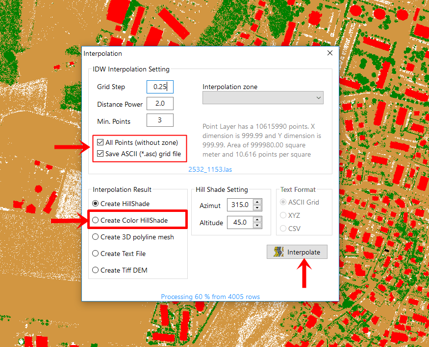
The simplest approach we provide with SGIS technology is to check the “Create Color Hillshade” box during the interpolation of a point cloud, which will automatically generate the hillshade.
Fig. 1 Illustration of the SGIS v.R interface, highlighting the "Create Color Hillshade" option. When users select this checkbox during the interpolation of a point cloud, the system automatically generates a color hillshade, streamlining the process for enhanced visualization of terrain features.
But, we also want to showcase additional options by providing practical examples that highlight the capabilities of SGIS v.R.
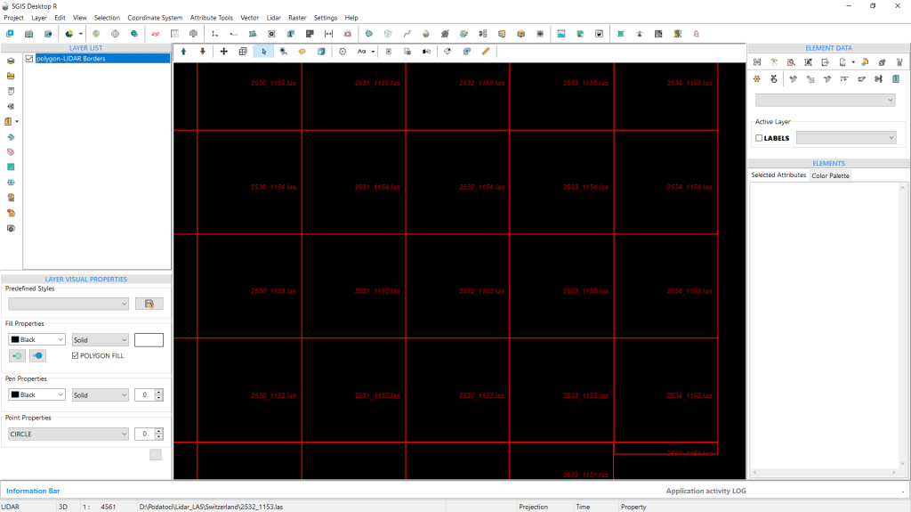
To demonstrate this, we loaded a LiDAR boundary grid, which will allow us to add a LAS point cloud.
Fig. 2 Display of the LiDAR boundary grid loaded into SGIS v.R software.
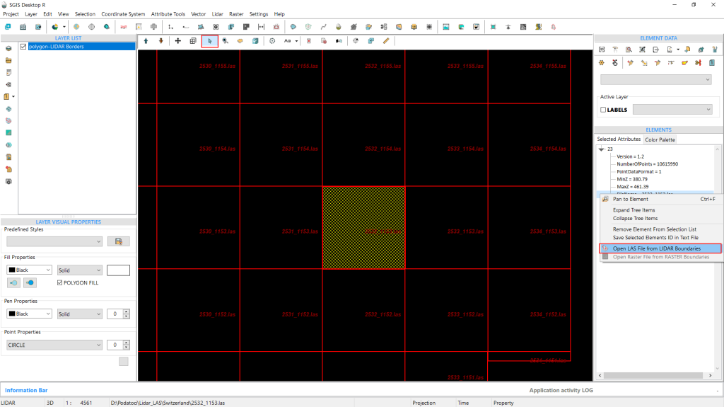
Fig. 3 Screenshot of the styled LiDAR boundary grid within the SGIS interface, featuring visible file names for better clarity. The background has been set to a dark color to enhance visibility. The image illustrates the process of selecting a LAS file from the ‘Elements’ toolbox, demonstrating the right-click submenu and the function used to open the selected file for further analysis.
We styled the LiDAR boundary grid earlier to show the file names, making it easier for us to understand and locate our data.
We also changed the background to a darker color. Now, we can select the desired LAS file and right-click on a row from the ‘Elements’ toolbox to open it. The LAS point cloud is loaded right away.
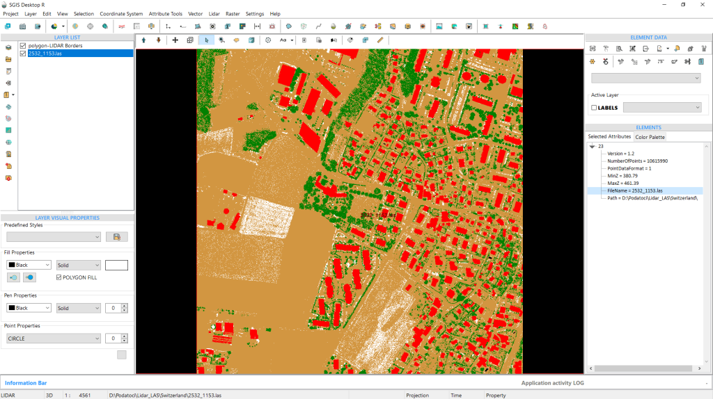
Fig. 4 The LAS point cloud data is integrated into the project.
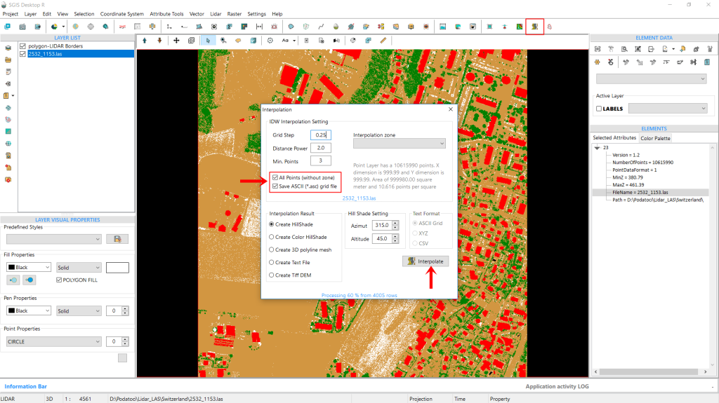
Next, we’ll adjust the interpolation parameters. We’ll set the Grid Step to 0.25m, the Distance Power to 2, and the Minimum Points to 3. Additionally, we’ll check the boxes for ‘All Points’ and ‘Save ASCII’, which we’ll explain further along in the process.
Fig. 5 Setting the interpolation parameters in the SGIS interface. The checkboxes for ‘All Points’ and ‘Save ASCII’ are selected, also the default ‘Create Hillshade’ option remains enabled in the Results tab before clicking on ‘Interpolate’.
We’ll also keep the default setting for ‘Create Hillshade’ in the Results tab. Once everything is set, we click on ‘Interpolate’.
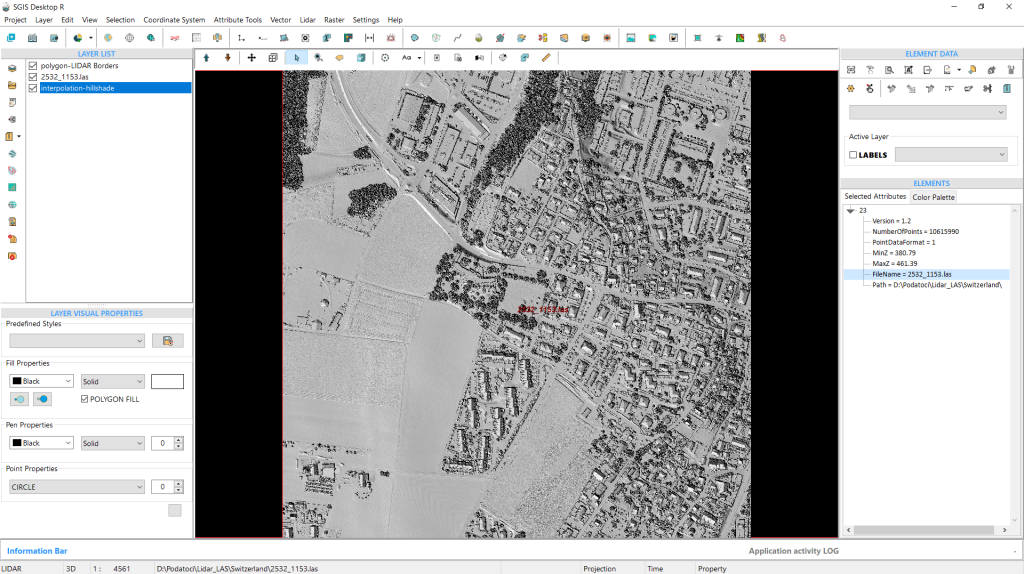
We’ve detailed this process in our document titled “[Developing Algorithm for Creating a DEM Grid from LiDAR Point Cloud Based on IDW Spatial Interpolation in SGIS v.R – Interpolating LIDAR Point Clouds to Raster with IDW with SGIS v.R].” The outcome of this interpolation is the generation of the hillshade DEM, which is reflected in the new layer that appears instantly in the ‘Layers List’ panel.
Fig. 6 The result of the interpolation process is the generation of the hillshade, displayed as a new layer in the ‘Layers List’ panel of the SGIS interface.
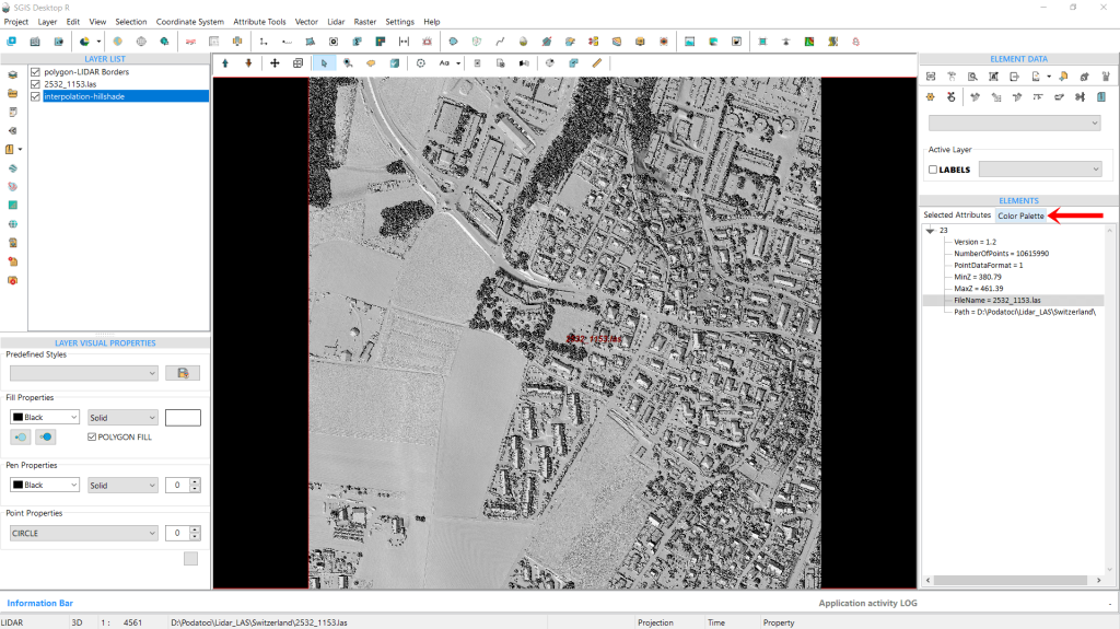
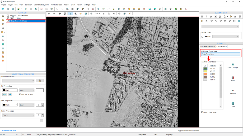
Fig. 7 Navigating to the ‘Color Palette’ tab within the ‘Elements’ panel to adjust the color settings for the color hillshade layer we'll create next.
Now that we’ve completed this step, we’ll move to the ‘Color Palette’ tab under the ‘Elements’ panel.
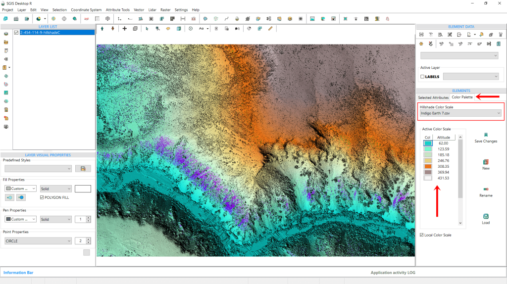
This tab offers a visual color scale ramp, as well as several other tools. We’ll start with the ‘Hillshade Color Scale’ dropdown, where we can select a preferred color scale. SGIS includes multiple preset color ramps, and users can also add custom color scales. In Fig. 8, we see a preset called ‘Earth Tone 5,’ which consists of five colors, each adjusted to specific elevation values displayed below the dropdown.
Fig. 8 The ‘Hillshade color scale’ dropdown menu is shown, displaying the ‘Earth Tone 5’ preset.
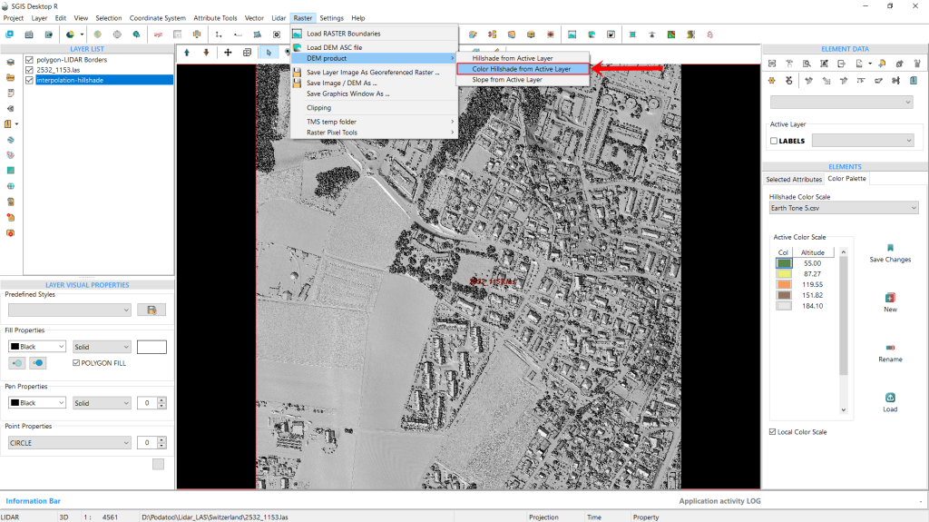
To demonstrate the simplicity of this feature, we’ll leave the color scale as-is, using the default ‘Earth Tone 5’ preset. For users working with a preloaded DEM-hillshade without a LAS file, SGIS provides this second option to create a Color Hillshade directly from the ‘Raster’ menu by simply selecting a preset color scale.
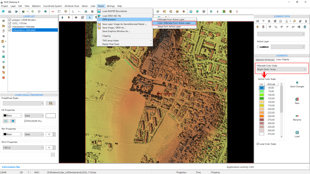
Since we’ve now completed the creation of our example hillshade process, and the hillshade layer is visible in the ‘Layers List’, we’ll navigate to the Raster menu, go to ‘DEM Products’, and select ‘Color Hillshade from Active Layer’. Clicking on this immediately generates the color hillshade as a new layer in the Layers List.
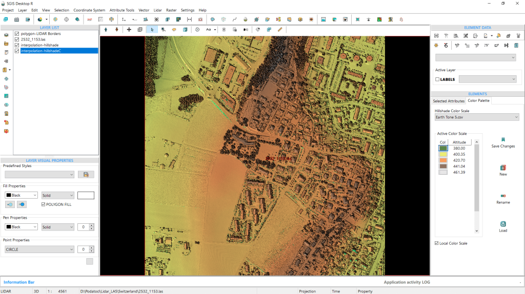
Additionally, users can choose to display their data with either a local or global elevation scale. In our example, we’ve used the local scale option, which provides a tailored representation based on our specific terrain. This new color hillshade DEM layer reveals a clear contrast to the regular hillshade, making it easy to identify variations in elevation.
With color, it’s much easier to distinguish high and low areas, enhancing both depth and elevation, and terrain detail.
Fig. 9 Applying a preset color scale for color hillshade creation. SGIS offers a streamlined option to create a Color Hillshade directly from the ‘Raster’ menu for users with a preloaded DEM-hillshade layer.
Fig. 10 The generated color hillshade layer is displayed in the Layers list, indicating successful creation and ready for further customization or analysis.
The color hillshade is now generated, and its layer appears in the Layers list.
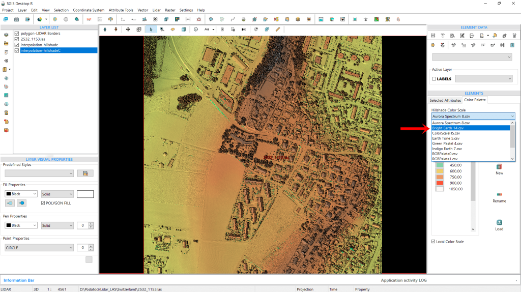
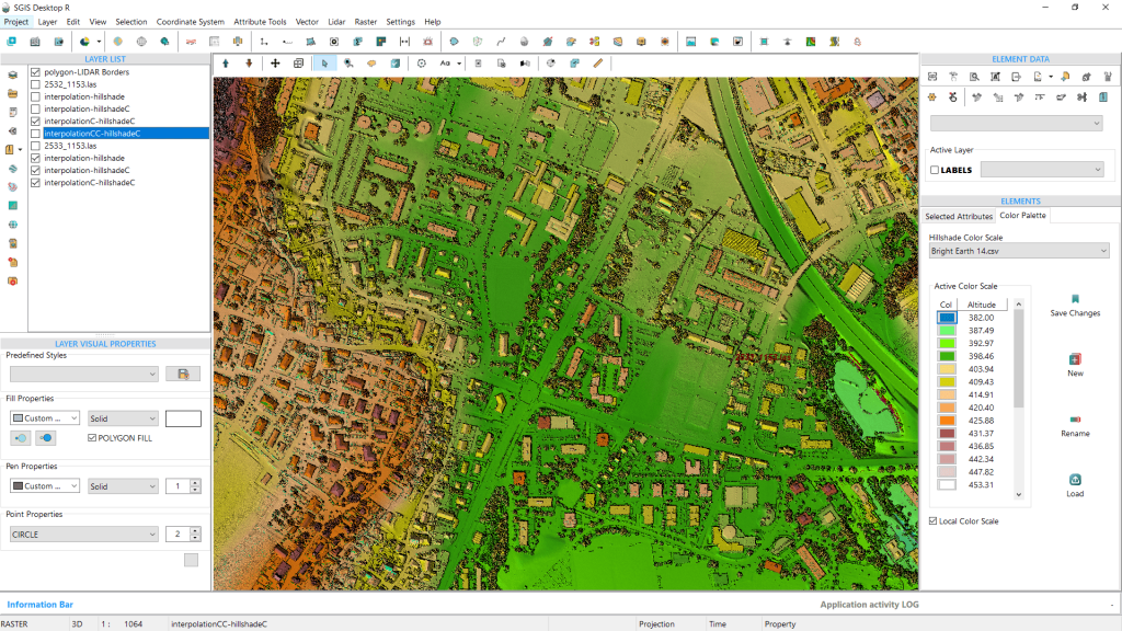
If we want to change the color scale, we can easily do so by opening the dropdown menu and selecting a different preset. For this example, we’ll select the ‘Bright Earth 14’ palette. The “14” here represents the number of elevation intervals in the preset, meaning it uses 14 distinct colors to represent varying elevations.
Fig. 11 Changing the color scale for the color hillshade layer by selecting the ‘Bright Earth 14’ preset from the dropdown menu, allowing for further customization of the visual representation.
Fig. 12 Selecting a new color scale from the dropdown list and clicking on the ‘Color Hillshade from Active Layer’ option to apply the updated color settings to the hillshade layer in SGIS v.R.
To apply the change, we simply need to select the desired preset from the list and then click on the ‘Color Hillshade from Active Layer’ option again. This action will create a new color hillshade layer, which will appear in the list of layers.
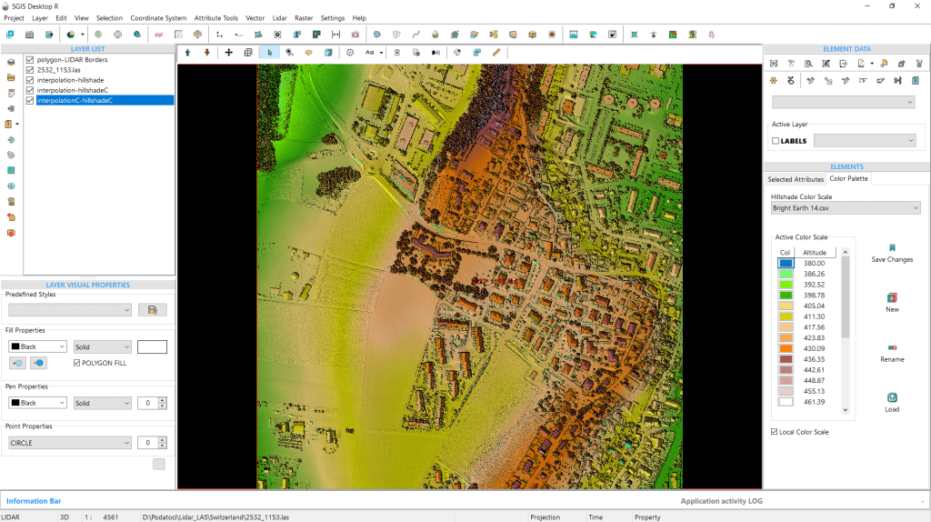
This updated representation provides a more intuitive view, showcasing the elevation changes in the terrain with greater detail.
Fig. 13 The ‘Bright Earth 14’ preset color scale, which utilizes 14 distinct colors to represent different elevation intervals, enhancing the visual differentiation of elevation levels in the color hillshade layer.
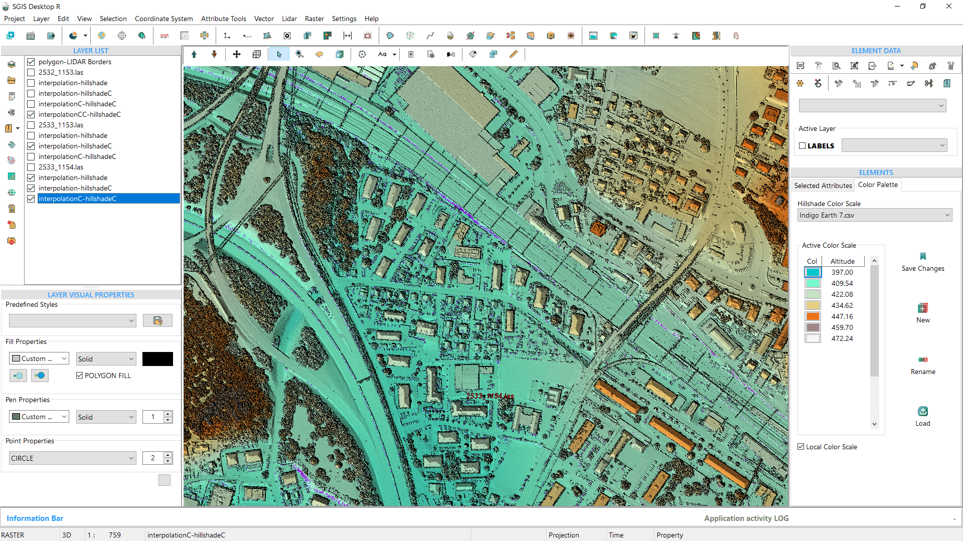
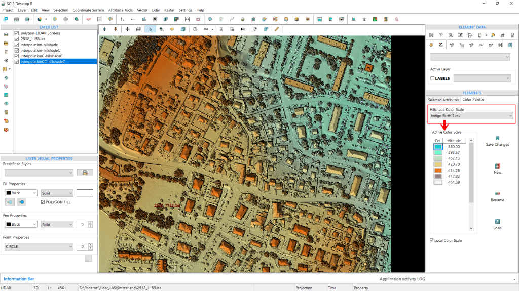
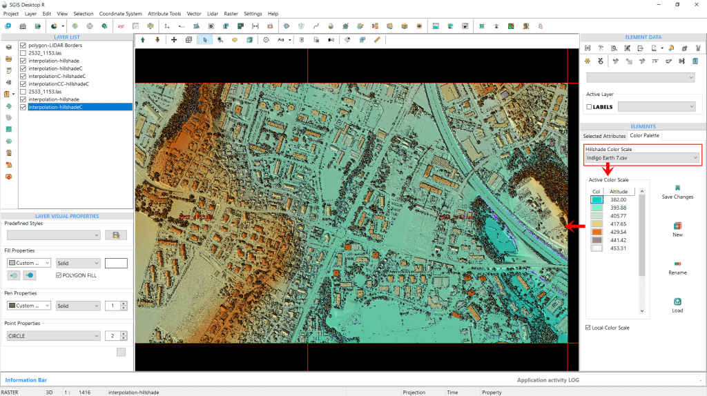
To highlight some of our presets, we’ll go through the process again, this time using the ‘Indigo Earth 7’ color hillshade scale. The outcome of this selection is displayed in Fig. 14.
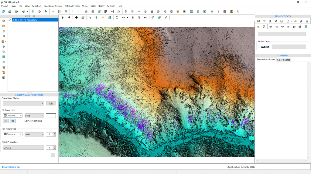
Fig. 14 The result of applying the ‘Indigo Earth 7’ color hillshade scale.
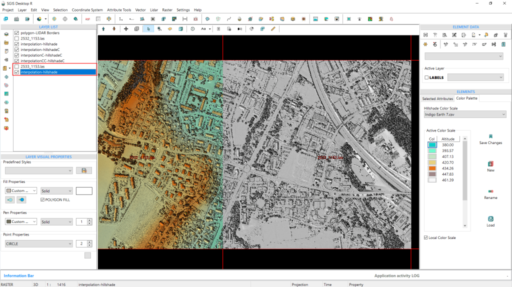
We’re going to repeat the entire process to highlight the potential benefits for users working on large-scale projects that involve multiple LAS files, or DEMs (DEM hillshades). By demonstrating how colorizing hillshades according to their elevation values enhances terrain visualization, we aim to show just how much more intuitive and informative the resulting maps can be.
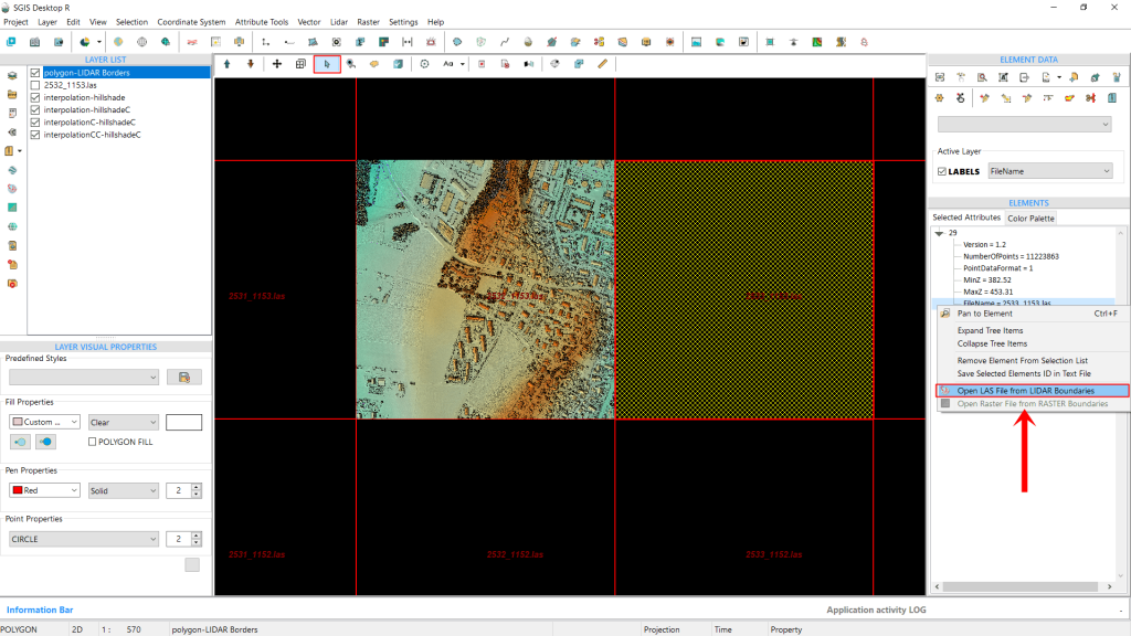
To accomplish this, we’ll choose the LAS file that is adjacent to the one we’ve already processed. First, we select the LiDAR boundaries layer, then click inside the grid square. After that, we can right-click to open the submenu and load the LAS files from there.
Fig. 15 Selecting the adjacent LAS file to the already processed layer by first choosing the LiDAR boundaries layer and clicking within the grid square. The submenu is opened with a right-click to load the new LAS file.
To make the process quicker, we’ve already created the hillshade. Now, we simply need to select the same ‘Indigo Earth 7’ color scale palette for both layers so they visually blend together (HS DEM 1 and HS DEM 2).
Fig. 16 Applying the same color scale palette to the newly created hillshade.
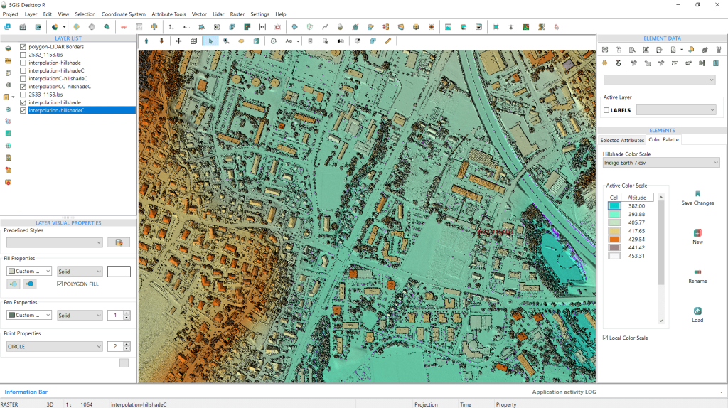
Fig. 17 The color hillshade displays a seamless transition between both DEM layers, creating a unified and detailed view of the terrain. Elevations are color-coded from indigo for the lowest areas to lighter orange-brown tones for the highest, clearly illustrating elevation changes across the landscape.
In Fig. 17, we see the smooth transition and seamless blending of both DEMs into a single, cohesive image, offering a vivid representation of the terrain.
The elevation color ramp shows the lowest areas in indigo blue, with elevation gradually increasing toward the left and right sides. This detail is far more discernible than with a standard gray hillshade.
Fig.18 This color enhancement provides a more intuitive understanding of terrain features compared to a standard grayscale hillshade.
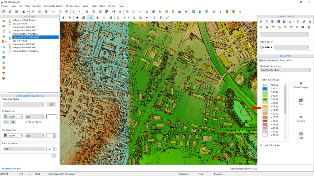
Fig. 19 Applying a new color ramp to one of the DEM hillshade layers while keeping the original ramp on the other.
We can also adjust the color ramp for one DEM hillshade while keeping the original for the other, or modify both for a cohesive visual effect. Using a different color ramp allows for a more nuanced depiction of elevation changes, enhancing terrain detail.
Fig. 20 Adjusting both DEM hillshade layers to use a unified color ramp for a cohesive view, enhancing the depiction of elevation variations and providing detailed terrain visualization.
We’ll demonstrate now how to create a color hillshade DEM by directly loading an ASCII DEM file (.asc grid file) into SGIS v.R.
An ASCII DEM (Digital Elevation Model) is a type of file format that presents elevation data in a simple text form. The term “ASCII” refers to the American Standard Code for Information Interchange, indicating that the information is stored using standard text characters. These files usually contain geographic coordinates along with elevation values arranged in a grid format. Each line represents specific elevation data points, collectively creating a digital model of the terrain.
In GIS applications, ASCII DEM files are frequently utilized for tasks such as terrain analysis, visualization, and generating models like hillshades. Their text-based format makes them easy to read and compatible with a variety of software platforms.
That’s why we checked the ‘Save ASCII’ checkbox in the interpolation dialog window earlier. If users have a LAS point cloud and want to save the data in a more shareable DEM Grid format, they can easily do so while generating the hillshade with those settings translated into the ASCII DEM Grid as well. The ASCII file will automatically be saved in the same folder as the original LAS data files, making it convenient to access and share.
Since using the exported dataset would yield the same results as before, we’ll use a different .asc file for this demonstration. This will allow us to explore the additional tools available in the ‘Color Palette’ tab.
We’d also like to explore the creation of colored hillshade for undulating terrain with mixed forest cover.
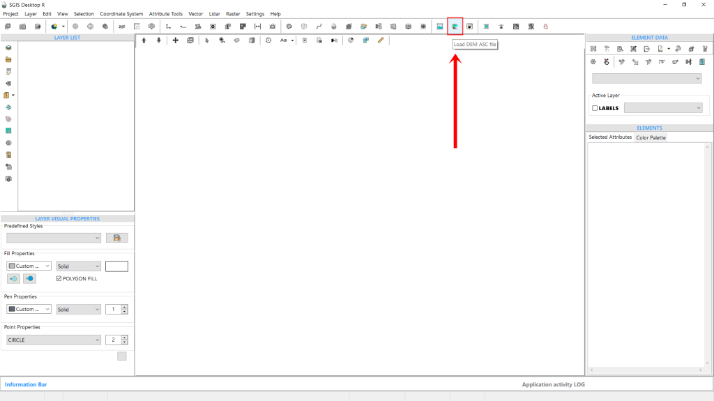
Fig. 21 Accessing the 'Load DEM ASC file' function from the main ribbon bar in the SGIS interface. This feature provides quick access to load DEM files directly into the project for further customization and analysis.
Let’s begin by locating the ‘Load DEM ASC file‘ function, conveniently placed in the main ribbon bar of the software interface for quick access.
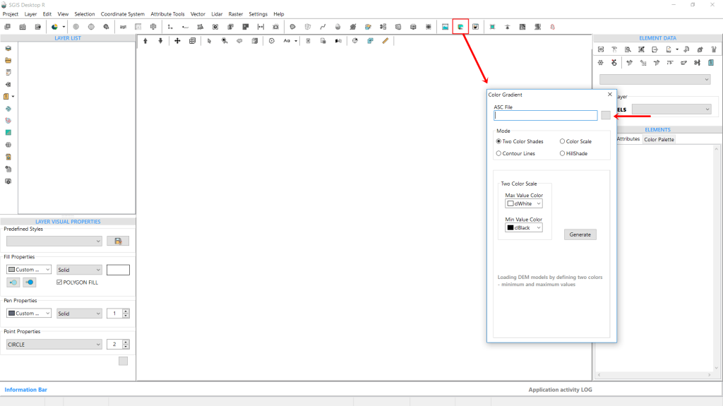
After selecting it, a new dialog window opens, prompting us to configure some settings for our task. First, we’ll define the file path to locate our desired DEM file.
Then, we’ll set the ‘Mode’. Currently, there are four modes to choose from:
Two-Color Shade;
Color Scale;
Contour Lines;
and Hillshade.
We’ll walk through each mode with practical examples later, but for now, we’ll stick with this demonstration and select the fourth option by checking the Hillshade checkbox.
Fig. 22 Configuring the DEM loading settings in SGIS. The dialog window allows users to specify the file path and select from four modes: Two-Color Shade, Color Scale, Contour Lines, and Hillshade, based on their visualization needs.
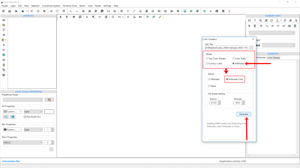
Comparing Fig. 22 and Fig. 23, we can see that by default, the function opens with the ‘Two-Color Shade’ mode selected. However, when we switch to Hillshade by checking its box, the menu adjusts to show new options. In the original view, users can adjust settings specific to ‘Two-Color Shade,’ but with Hillshade selected, the “Result” box offers three options:
Hillshade,
Color Hillshade,
and Slope.
For this example, we’ll select Color Hillshade.
Below this, additional hillshade settings for Azimuth and Altitude appear, set by default to 315° and 45° respectively. With everything configured, we just need to click ‘Generate’ to complete the process.
The color hillshade DEM is instantly created as a new layer and displayed in the graphics panel.
Notably, we previously set the color scale palette to ‘Indigo Earth 7,’ so the software automatically applies this palette as the default for any new color hillshades generated unless it’s changed.
Fig. 23 Adjusting hillshade options after switching from the default ‘Two-Color Shade’ mode to Hillshade. Selecting the Hillshade option modifies the menu to display new settings, including the "Result" box with Hillshade, Color Hillshade, and Slope options. Here, Color Hillshade is selected. Additional controls for Azimuth (default 315°) and Altitude (default 45°) provide further customization for the final visualization.
Fig. 24 Generated color hillshade DEM layer displayed in the graphics panel. The color scale palette ‘Indigo Earth 7’ is automatically applied, as it was set previously, becoming the default for any newly created color hillshades unless manually updated.
We’d also like to go over the tools available in the ‘Color Palette’ tab, which allow users to adjust and manipulate color scales for enhanced visualization.
Fig. 25 Tools available in the ‘Color Palette’ tab for adjusting and manipulating color scales to enhance visualization.
Earlier, we covered how to change the color scale by selecting from the dropdown list, which includes some preloaded SGIS presets. However, users can further customize the color scales using the tools on the right side of the toolbox. Let’s now go over each of these tools in detail.
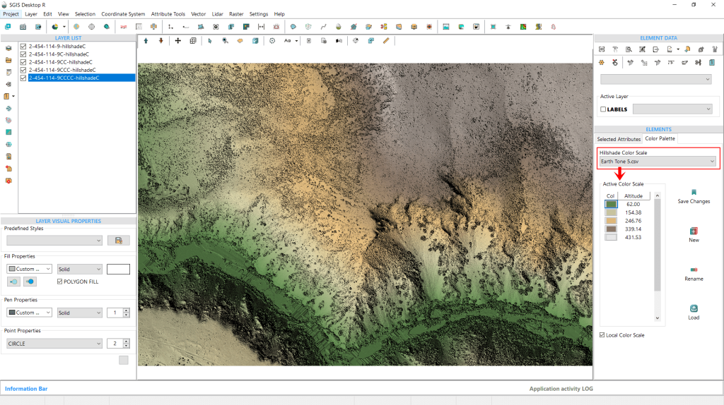
Fig. 26 Changing the color scale preset to 'Earth Tone 5' with fewer elevation intervals. The color values for each elevation interval are displayed, allowing further customization.
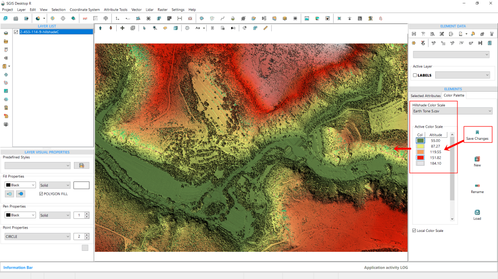
We’ve changed the preset, as shown in Fig. 26, selecting one with fewer elevation intervals, ‘Earth Tone 5.’ In this view, we can also see the color values assigned to each elevation interval. To modify these, simply click on the color rectangle. A color palette will pop up, allowing us to pick a new color for that particular elevation.
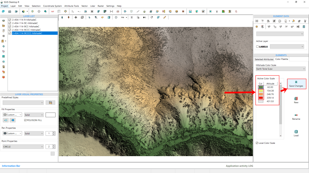
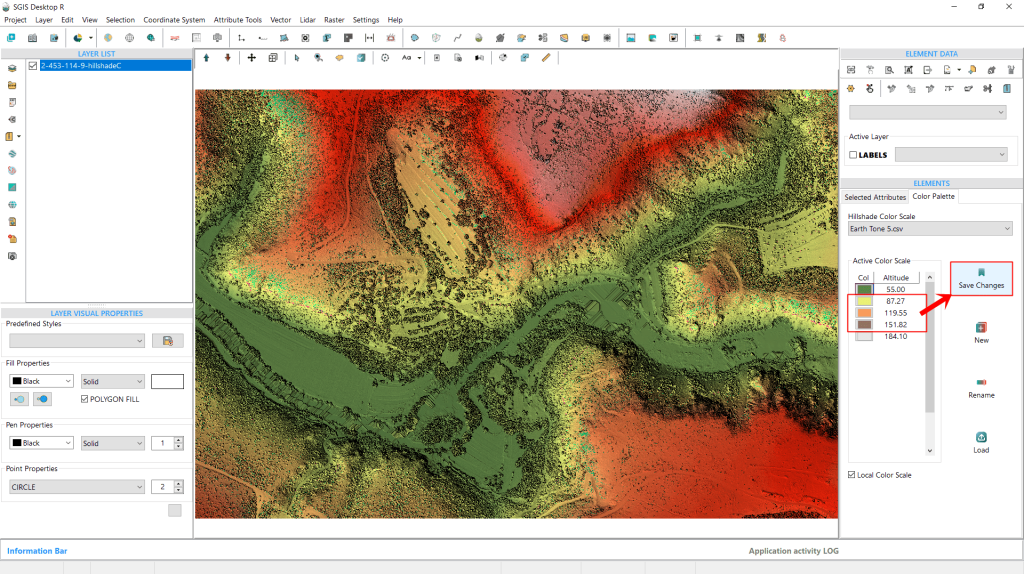
For this example, we’ve decided to update the colors of the three middle elevation values within the ‘Earth Tone 5’ scale. To save these changes, all we need to do is click the ‘Save Changes’ button on the right side.
Fig. 27 Customizing the colors of the three middle elevation values within the 'Earth Tone 5' scale. Changes are saved by clicking the 'Save Changes' button.
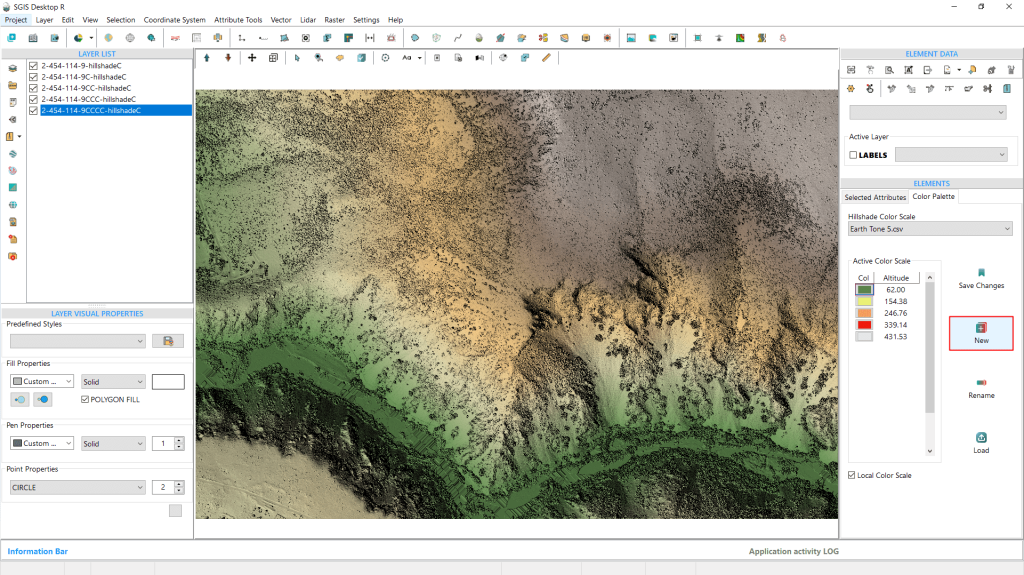
Fig. 28 Creating a new preset scale by using the ‘Create New’ option. The new scale is saved and can be accessed later through the dropdown list for future analysis.
The next function, ‘New’, lets users create a custom preset by entering minimum and maximum elevation values in a dialog window and specifying the number of intervals they want for the custom scale.This new scale will then be available for future use in the dropdown list for further analysis.
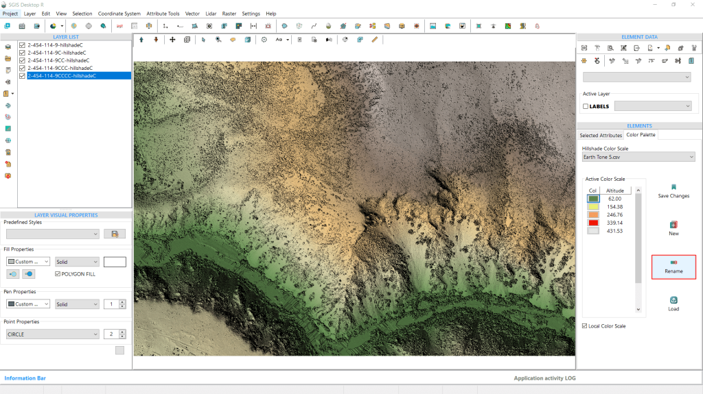
Fig.29 The "Rename" feature allows users to personalize color scales by assigning custom names, enhancing organization and making it easier to find and remember preferred presets.
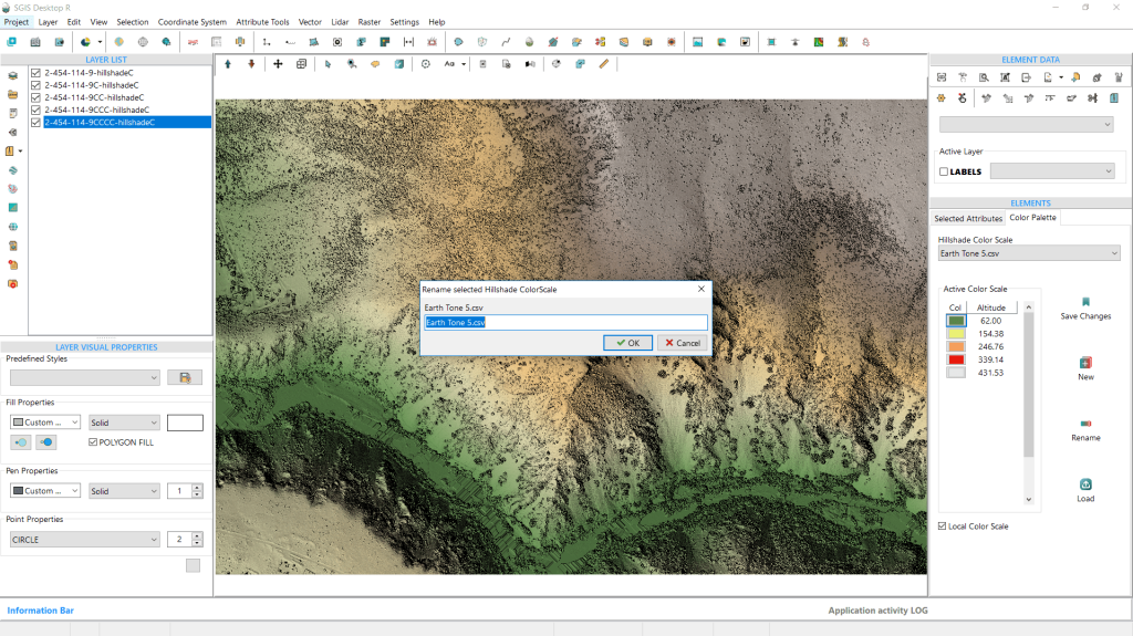
The third option is the “Rename” feature, which allows users to rename color scales for better organization and personalization. This is particularly useful for customizing presets, enabling users to give them names that are easier to remember or align with their preferences.
Fig.30 Upon clicking "Rename," a prompt appears allowing us to enter a new name for the preset.
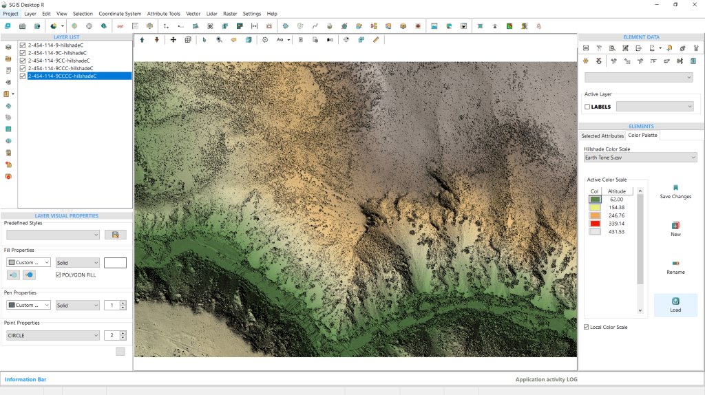
Fig.31 The 'Load' feature allows users to import a predefined text file containing custom color settings, where each row defines an elevation value along with its corresponding RGB color values.
The final option is the ‘Load’ feature, which allows users to import a predefined text file containing their own color settings. The file should follow this format: ‘elevation value;R;G;B’, with semicolons separating each value. This means the file will have four columns, and users can define the number of rows, with each row representing a specific elevation value.
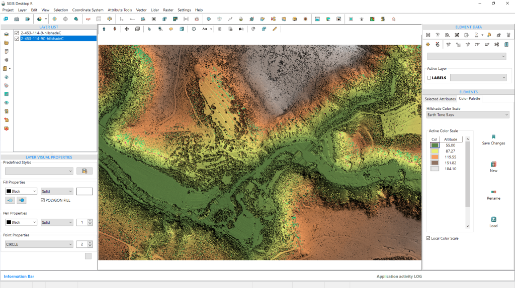
Fig.32 Demonstrating the updated color scale, with a newly created color hillshade DEM based on the previously modified settings.
To wrap up our procedure, we’ll demonstrate the updated color scale that we previously modified. We’ve created another color hillshade DEM based on these settings. Now, we’ll switch the colors back to more subtle tones and save them once again.
This color hillshade DEM can later be exported in various formats, including DEM TIFF, Raster TIFF, JPG, PNG, or other available georeferenced raster formats.
Fig.33 Reverting the color scale to more subtle tones before saving the changes.
Fig.34 The color hillshade DEM can later be exported in various formats, including DEM TIFF, Raster TIFF, JPG, PNG, or other available raster options.