Elevation-Based Segmentation of Point Cloud Data: Extracting LAS Datasets by Defined Elevation Ranges (e.g., 0-2m, 2-5m, 5-10m) within a particular ASPRS classification
Published on: 26.10.2024
Elevation-based segmentation of point cloud data—where LAS datasets are filtered by specific elevation ranges—allows for a more targeted analysis of vertical layers within a landscape. By creating these distinct elevation bands, users can easily focus on specific vertical sections, like the ground surface, vegetation, buildings, or utility poles, which simplifies the analysis of complex terrain features.
This approach also makes data handling and processing more efficient. By narrowing in on only the relevant elevation bands for a particular task, we can reduce processing loads and focus computational power on the most critical areas, resulting in faster and more streamlined analyses.
There are many practical applications for this type of segmentation, and we’d like to highlight a few that demonstrate its practical benefits. One especially valuable use case is isolating elevation bands from LAS files for focused analysis.
For instance, we have a real-world scenario where the client needs to assess the natural slope of the terrain at a specific site to plan the installation of a sewer line. They want to connect the building to a point along the main sewer line, and by using point cloud data, we can determine the quickest and simplest route for this installation. By extracting only the ground points within the desired elevation range, we can provide the exact information needed for the task.
Another example involves extracting low-lying vegetation points from a relatively flat terrain or isolating tall building structures in an urban point cloud filled with various buildings. Each of these applications highlights the usefulness of segmentation by elevation in point cloud analysis.
We’ll demonstrate how this is done using SGIS v.R.
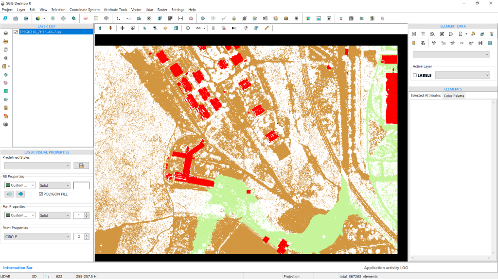
Fig. 1 Dataset Loaded in SGIS v.R.
We’ve already loaded our LAS file. As shown in the graphics panel, the data includes classifications for ground, buildings, and other points marked as unclassified or class 1 according to ASPRS standards, as well as low points. This setup works well for our needs, as we’re primarily interested in the ground points for further data processing.
In SGIS v.R, the in-built ‘Statistics’ memo provides valuable data insights. Here’s how it works:
Once the LAS file is displayed, we activate the selection function. Using the mouse cursor, we click on a specific area of the point cloud at an appropriate zoom level—not too close—so we can select a group of points. By pressing CTRL+S, the ‘Statistics’ memo opens.
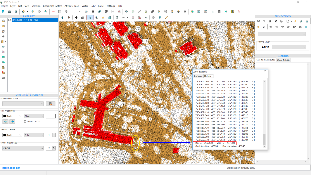
This memo box contains two tabs: ‘Statistics’ and ‘Details.’ We’ll open the ‘Details’ tab. Scrolling down to the end of the list, we’ll find information about minH and maxH, which indicates the minimum and maximum elevations within the selected points. This tells us the elevation range for that particular cluster of points.
With this elevation data, we’ll know the exact range to input in the ‘Elevation Range’ selection process. In our case, we’ll take note of 257.5m H and move forward with processing.
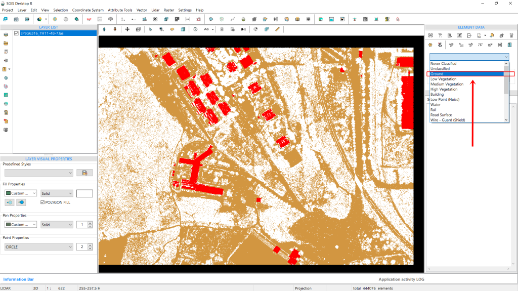
Next, we’ll close the Statistics window. Below the ‘Element Data’ toolbox, there’s a dropdown menu displaying various classifications. From here, we’ll select “Ground” points. This means that any selection procedure or function we apply will target only the ground points, not the entire point cloud. If we had chosen class 1, for instance, the selection would focus specifically on those class 1 points instead.
Fig. 2 In the Element Data toolbox dropdown menu, "Ground" points are selected, ensuring that subsequent functions or selections apply exclusively to ground points within the point cloud rather than the entire dataset.
Next, we’ll navigate to the Selection menu and choose ‘Select Elements by Elevation Range’.
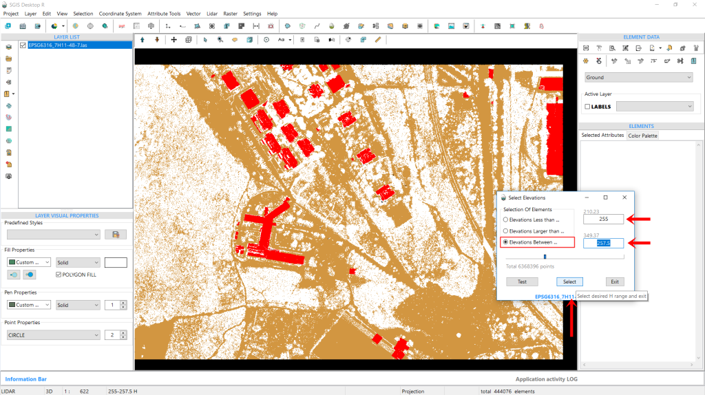
Then, we’ll check the third box labeled ‘Elevations between…’ As soon as we click on this option, the input boxes on the right become active. In the first box, we’ll enter H 255 m, and in the second box, we’ll enter H 257.5 m. This setup means we want to highlight and select all ground points with elevations ranging from 255 to 257.5 m.
Finally, we’ll click on ‘Select’ to proceed.
Fig. 3 From the ‘Select Elements by Elevation Range’ window, the third checkbox labeled ‘Elevations between…’ is checked, activating the input boxes, allowing the user to enter elevation values of H 255m in the first box and H 257.5m in the second box to highlight and select ground points within this range.
Fig. 4 All points that meet the specified criteria are selected and highlighted in green, illustrating the effective application of the selection process; the highlight color was changed from the default red to green for improved clarity, particularly to avoid confusion with red-colored buildings.
As shown in Fig. 4, all the points that meet this criteria are now selected and highlighted. For clarity, it’s important to mention that we previously changed the highlight and selection color to green. The default red color wasn’t suitable for several other previous projects, where we needed to highlight buildings that were also red.
This is a customizable option that users can modify according to their preferences.
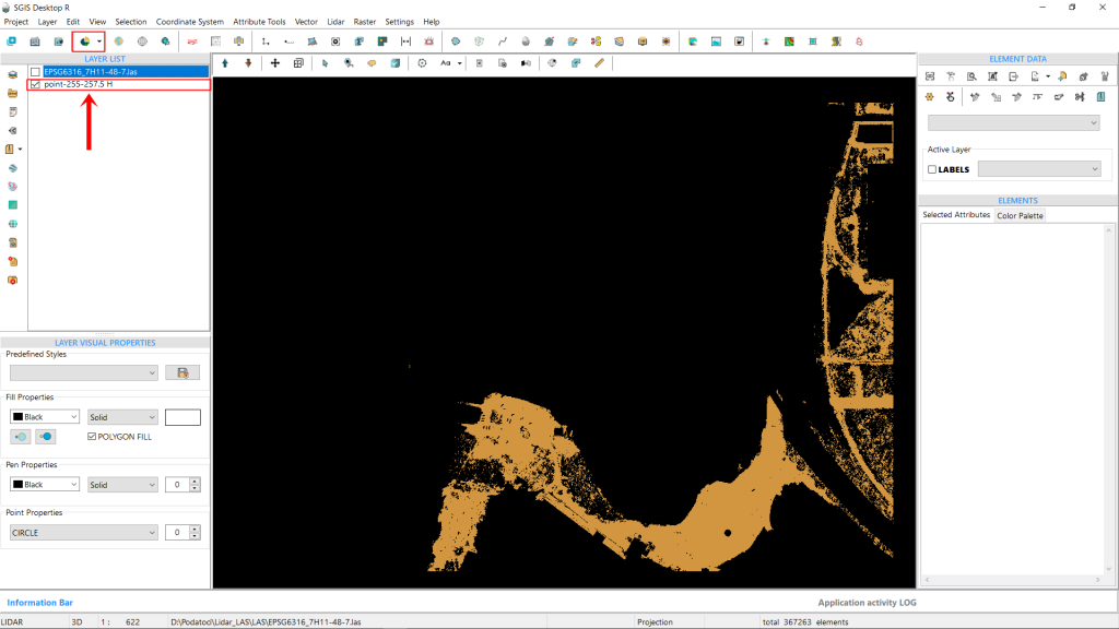
Next, we’ll use the ‘Selected Elements in New Layer’ function to separate these points into a new layer, which we’ll name “points 255-257.5 H.” If we create multiple layers for different elevation bands in the Layers panel, giving them clear names will help us keep track of everything during our processes.
Fig. 5 The ‘Selected Elements in New Layer’ function is used to create a new layer named "points 255-257.5 H," allowing for better organization of the point cloud data; clear naming of multiple layers for different elevation bands in the Layers panel aids in tracking and managing the data throughout the analysis process.
This extracted point dataset can later be saved as a separate LAS file, or in TXT, CSV, ASCII, or XYZ formats. In our specific case, this means we have the ground elevations from the desired point A to point B, allowing us to create profile sections and conduct further analysis. Additionally, since this dataset contains significantly fewer points than the entire point cloud, it reduces the strain on hardware during subsequent processing.
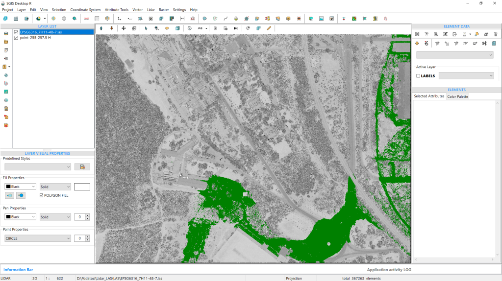
To get a clearer view, we’ll enable both layers from the Layers panel. The first layer will display the entire point cloud, which we’ll set to Intensity view mode. We’ll also change the color of the extracted ground points for better visibility.
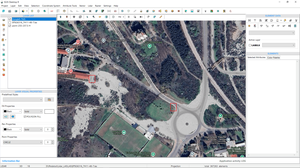
Alternatively, we can disable the entire LAS point cloud and add a Tile map layer as a backdrop, showing only the extracted points in Intensity view mode. This approach, illustrated in Fig. 7, is particularly useful because the intensity view allows us to clearly see features like roads and concrete surfaces.
Fig. 6 Both layers are enabled in the Layers panel, with the entire point cloud set to Intensity view mode and the color of the extracted ground points adjusted for enhanced visibility.
Fig. 7 The entire LAS point cloud is disabled, and a Tile map layer is used as a backdrop, displaying only the extracted points in Intensity view mode, which enhances visibility of features like roads and concrete surfaces.
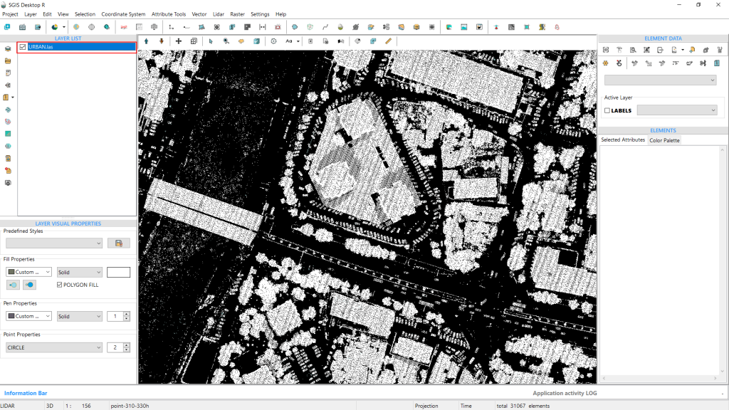
We’ll look at another example from a practical case with an urban point cloud. This LAS file includes multiple structures, such as houses and buildings, among which are three tall buildings that we’re focused on extracting for this example. Since this area is densely built, we need to carefully examine the elevation data to isolate the tallest buildings.
The point cloud has been imported, and we’ve already set the classifications using the ‘LiDAR’ toolbox. After reviewing the available classifications, we found only Ground, Unclassified, and Low points in this dataset. We’ve disabled all points except for classification 1. Since vegetation (low, medium, and high), unclassified points, and building points are all included under class 1, we first need to assess the elevation in our target area.
Fig. 8 An urban point cloud dataset showing multiple structures, including houses and buildings.
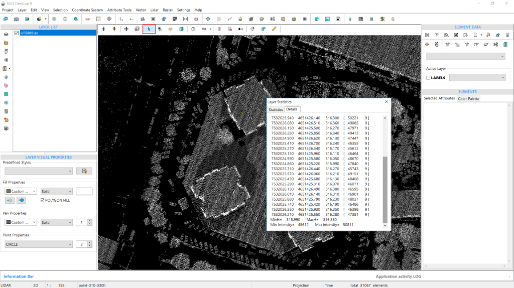
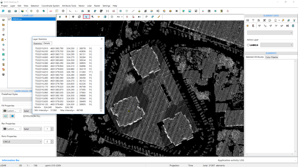
So, we’ll repeat the process by selecting clusters of points at several spots. Then, we’ll press CTRL+S, go directly to the Details tab, and scroll to the bottom to view the minH and maxH values. We’ll repeat this once more to ensure a precise elevation check.
Fig. 9 Clusters of points are selected around the target area, with minH and maxH values displayed in the Details tab to refine elevation accuracy.
Fig. 10 A second round of point selection and elevation check is performed to confirm precise minH and maxH values in the target area.
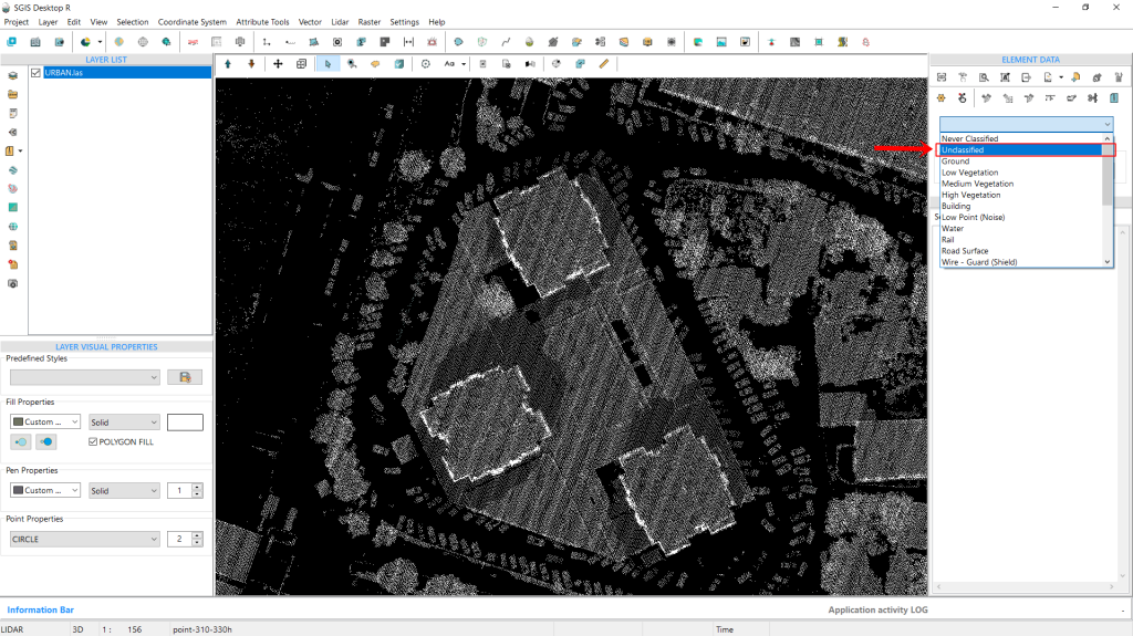
Fig. 11 The classification dropdown is set to “Unclassified,” indicating that only points within this classification will be selected in subsequent steps.
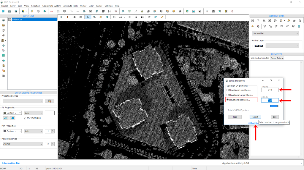
Once we’ve noted the necessary elevation values, we open the classification dropdown on the interface and select “Unclassified,” as we’ll be working with points from this classification. Next, we navigate to the Selection menu and choose “Select Elements by Elevation Range” once again. A dialog window appears, prompting us to set the parameters. We check the box labeled “Elevation Between…” and enter the desired elevation values. This time, we’ll specify a range from 310m to 330m. With these values in place, we click “Select” to continue.
Fig. 12 The dialog window for "Select Elements by Elevation Range" is displayed, with the box labeled “Elevation Between…” checked and the elevation values set to a range of 310m to 330m.
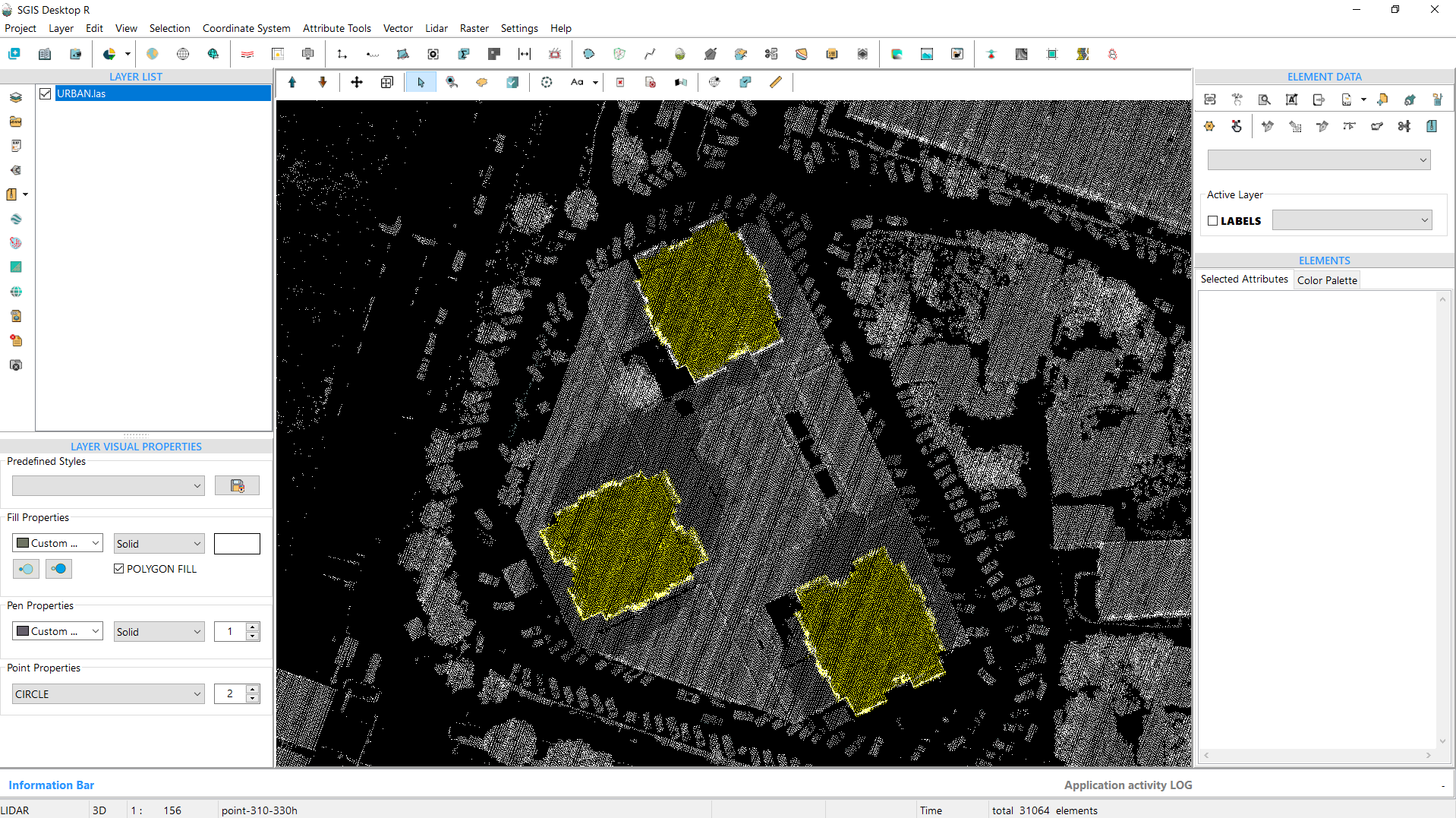
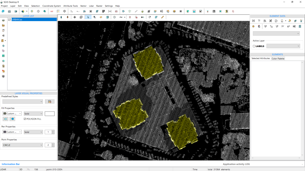
Fig. 13 The selected points are highlighted in a bright yellow color.
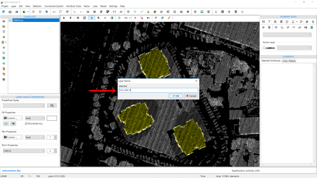
The points are instantly selected and highlighted in a bright yellow color. Next, we’ll isolate these points into a new layer using the ‘Selected Elements in New Layer’ function. When prompted, we’ll name this layer “points 310-330 H” to ensure clear distinction for future processing. After entering the name, we click ‘OK’ to create the layer.
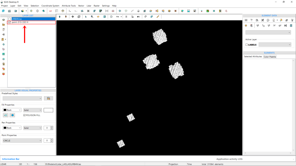
When we zoom out, we can see that, in addition to the three buildings we were targeting, two more buildings also fall within this specific elevation range. Since we don’t need these additional buildings, we can easily select and delete them. This is worth mentioning since we are selecting points from a specific ASPRS classification, but we’re still working with the entire point cloud. With that, we’ll wrap up our procedure.
Fig. 14 The points are isolated into a new layer named "points 310-330 H" using the 'Selected Elements in New Layer' function, ensuring clear distinction for future processing.
Fig. 15 Upon zooming out, it becomes evident that two additional buildings, aside from the three targeted structures, fall within the specified elevation range; these unnecessary buildings can be easily selected and deleted. With this the procedure is completed.