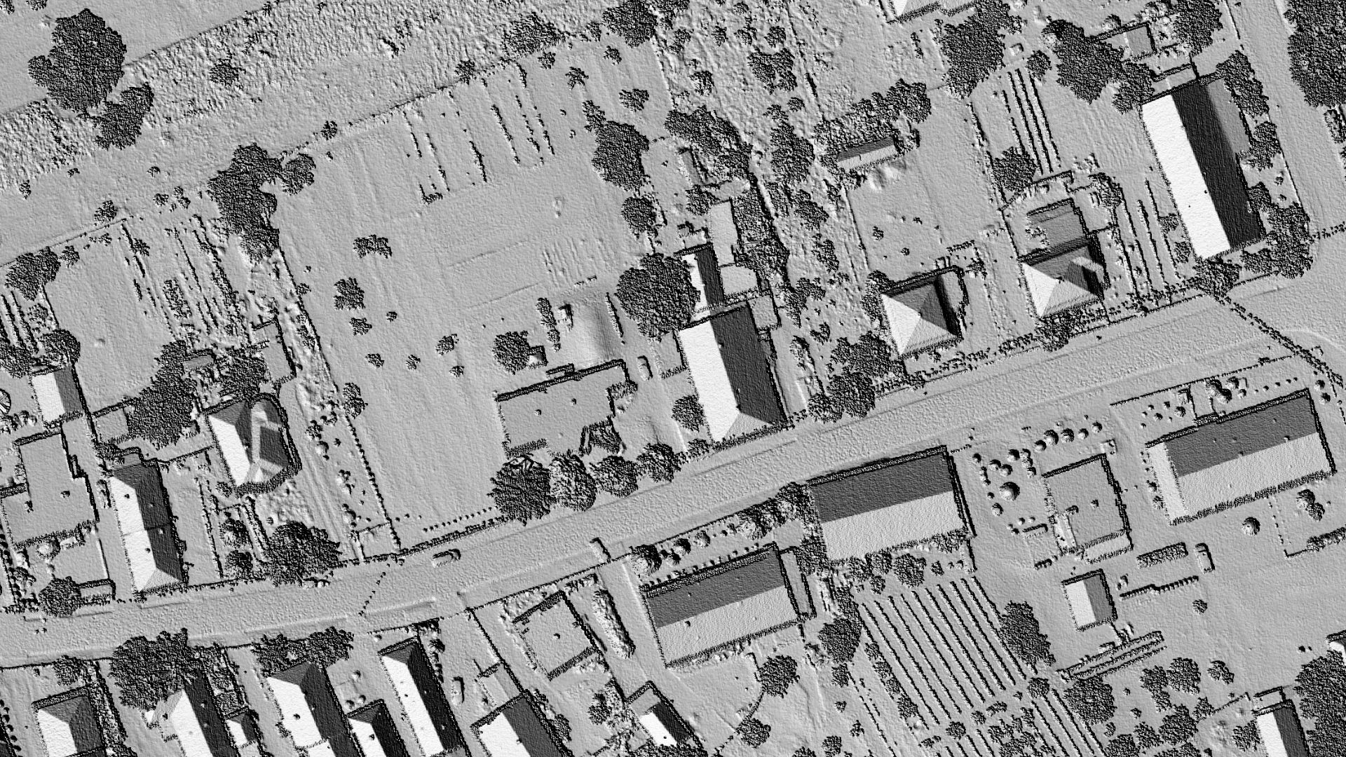
Developing Algorithm for Creating a DEM Grid from LiDAR Point Cloud Based on IDW Spatial Interpolation in SGIS v.R
Published on: 11.09.2024
As engineers, we often work with terrain data obtained through LiDAR technology, specifically LiDAR point clouds, which typically require various steps like corrections, reclassification, proper point assignment, and data cleaning to achieve accurate results. To streamline the process of visualizing terrain—without needing to clean the data upfront—and to assist in ongoing tasks, such as Quality Control, where terrain checks are essential, we developed our proprietary algorithm.
This algorithm is based on Inverse Distance Weighting (IDW) principles, offering a quick and precise solution for generating terrain models.
Spatial Interpolation
Spatial interpolation is a technique in Geographic Information Systems (GIS) that estimates unknown elevation values in unsampled locations using known data points from nearby areas. Essentially, it fills in the gaps where direct measurements are missing, allowing the creation of a continuous surface from discrete point data. This is particularly useful in terrain mapping, where we might only have elevation data for certain points. Spatial interpolation predicts elevation values in the spaces between, forming a complete Digital Elevation Model (DEM).
A DEM is a grid of squared cells (pixels), each assigned an elevation value (Manuel, 2004). Different interpolation methods applied to the same dataset can produce varying results, depending on the technique used.
These methods rely on the concept of spatial autocorrelation, which assumes that points closer to each other are more likely to have similar values than those farther apart.
Converting Sparse Point Data into Continuous Surfaces
Inverse Distance Weighting (IDW) is a common spatial interpolation method used to create continuous surfaces, such as Digital Elevation Models (DEMs) or hillshades, from LiDAR point clouds. LiDAR data consists of discrete points, each with specific coordinates and elevation values, but to perform meaningful terrain analysis—like generating hillshades or contour maps—a continuous surface is needed.
It’s worth noting that IDW works best when there are many elevation points in an area and they are dense enough to accurately represent local variations in the terrain.
The IDW method gives more weight to points that are closer to the area being interpolated, which is especially valuable for LiDAR data, as it captures localized terrain features more accurately. This makes IDW particularly effective for generating elevation surfaces that reflect actual terrain, even in regions where the density of LiDAR points may vary.
Another important note is that, LiDAR datasets can be incredibly large, often containing millions of points. IDW helps transform this vast data into more manageable grid-based surfaces, like DEMs or hillshades, which are easier to visualize and analyze in GIS software. Hillshades, typically generated from an underlying DEM created using IDW, offer a clear representation of terrain relief and slope. These visual models are crucial for understanding landforms, conducting environmental assessments, or planning various projects.
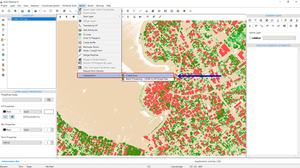
In SGIS v.R, this process is straightforward. To begin, we simply open the ‘Create Grid’ tool. Once selected, a new dialog window will appear.
Fig.1 Opening the ‘Create Grid’ function from the menu.
We’ve already imported the LiDAR point cloud, so now we’ll focus on explaining the settings and options within the function.
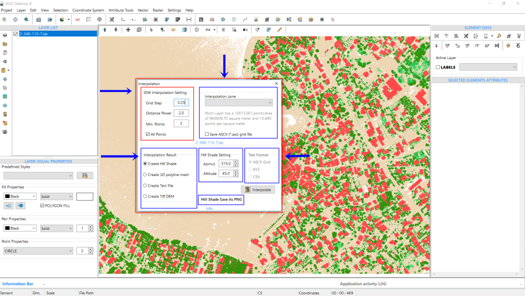
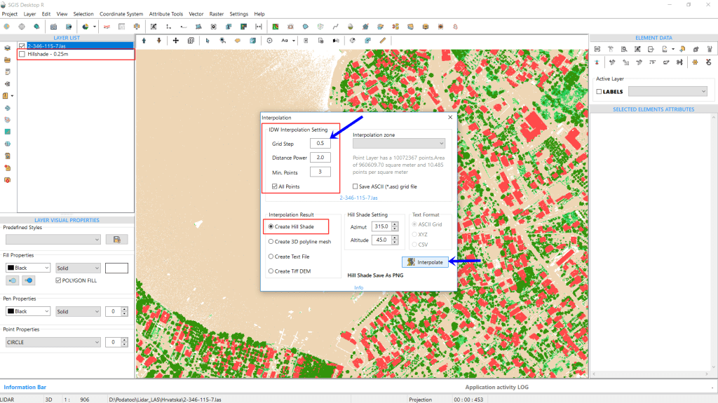
Fig.2 The IDW interpolation settings box allows users to customize parameters such as "Grid Step," "Distance Power," and "Min. Points".
In the ‘Interpolation Settings’ box, we can see that the point cloud contains 10,072,367 points, covering an area of 960,609.70 m², with average density of 10.485 points per square meter. This provides a sense of the data’s size, showcasing the efficiency of the algorithm, which completes the process in under a minute.
Moving to the settings, the first box includes the IDW interpolation parameters. Here, you’ll find an empty field for “Grid Step,” where users can input their preferred value (default is set to 1m). The “Distance Power” is set to 2 by default, though this can be adjusted as needed. The “Min. Points” option is set to 3 by default, and there’s also a checkbox labeled “All Points”.
For this example, we’ll set the “Grid Step” to 0.25m, while leaving the “Distance Power” and “Min. Points” at their default values of 2 and 3, respectively.
The next box in the settings is for defining the interpolation zone. If your input point cloud doesn’t have a fixed extent—meaning the points form an irregular shape—you’ll need to add a polygon layer and select it as the interpolation zone.
The ‘All Points’ checkbox and the ‘Interpolation Zone’ setting are key options, and users must select one or the other. If the area to be interpolated is rectangular, simply choose ‘All Points.’ However, for irregularly shaped areas, users need to add a Polygon layer (whether in Shapefile, GML, or GMT format) to the Layers Panel. Then, from the Interpolation Zone dropdown list, they can select the desired area (zone) for interpolation.
In this example, since we’re working with a fixed extent, we’ll leave this field empty. Below, there’s a checkbox labeled “Save ASCII” that allows users to automatically export an ASCII file (ASC Grid format file) from the process into the same folder. We’ll leave this unchecked as well.
At the bottom of the interpolation dialog, you can adjust the output settings. The first box lets users choose the type of output they want. You need to select one option before running the procedure. The options include generating a hillshade, creating a 3D polyline mesh, saving the output as a text file, or producing a Tiff DEM. On the right side, you can adjust the azimuth and altitude values for the hillshade—default values are 315 for azimuth and 45 degrees for altitude.
In this example, we’ve checked the first box to display the hillshade directly in the Layers Panel. If a user chooses to save the output as a text file, the third settings box will activate, offering format choices like ASCII grid, XYZ, or CSV.
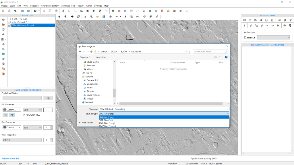
Additionally, the hillshade can be exported as JPG, TIFF, or PNG.
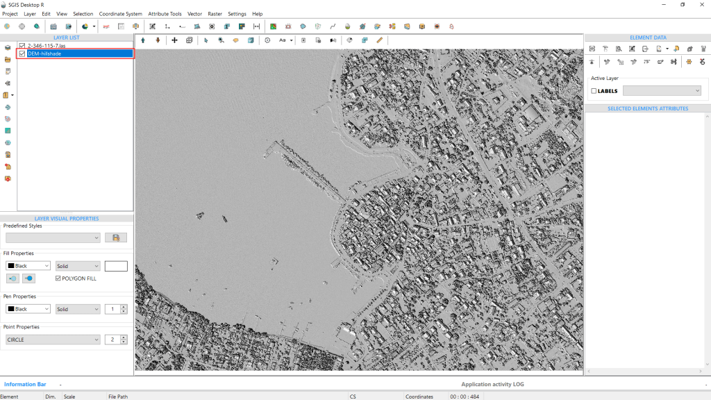
Once all desired settings are configured, we click “Interpolate” to run the procedure.
Fig.3 A hillshade with a 0.25m grid step has been generated.
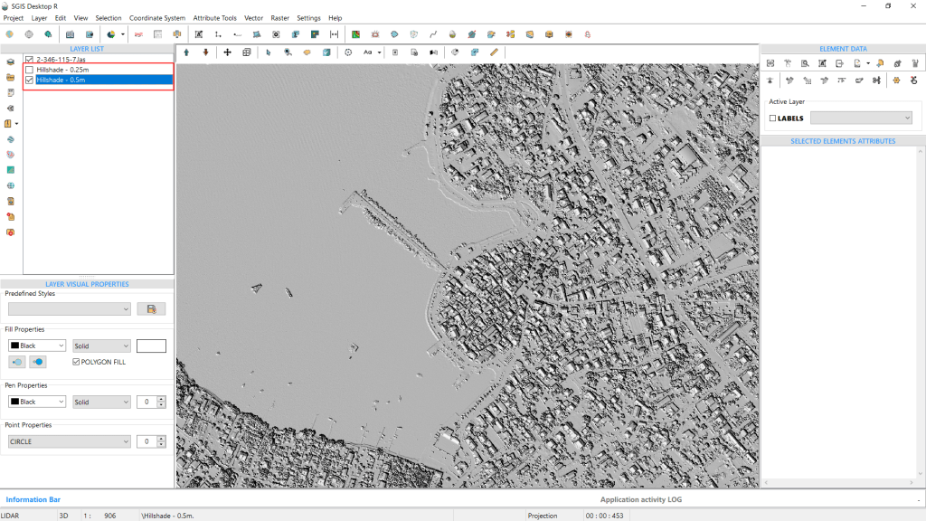
Fig.4 The procedure is repeated using a grid step of 0.5m.
We’ll run the process two more times to create hillshades with grid steps of 0.5m and 1m.
Afterward, we’ll compare the results of all three.
Fig.5 The second hillshade, created with a grid step of 0.5m, has been generated.
The process is repeated a third time, producing a hillshade with a grid step of 1m.
We will save all three hillshades as PNG files.
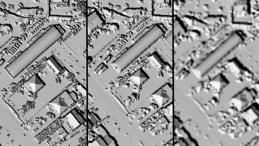
Fig.6 A comparison of the three hillshades at a specific location on the DEM.
In Fig.6, the difference in raster quality is clear. The first image highlights the hillshade with a 0.25m grid step, followed by the 0.5m grid step in the second image, and finally, the 1m grid in the third.
It’s evident that the sharpest and highest quality DEM is produced with the 0.25m grid step.
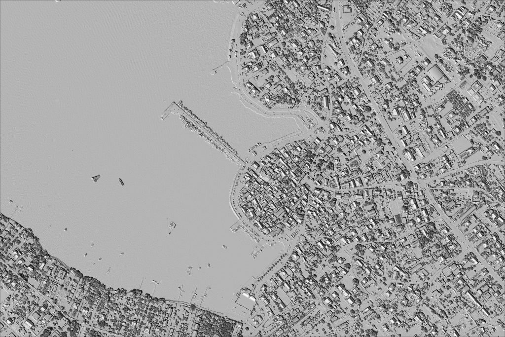
Fig.7 Hillshade DEM generated with a 0.25m grid step in SGIS v.R.
Fig.8 Hillshade DEM generated with a 0.5m grid step in SGIS v.R.
Fig.9 Hillshade DEM generated with a 1.0m grid step in SGIS v.R.
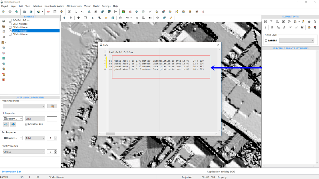
Fig.10 The LOG file showing the time taken for creating Hillshade DEMs with different grid steps: 1m took 25 seconds and 119 milliseconds, 0.5m took 12 seconds and 216 milliseconds, and 0.25m took 14 seconds and 497 milliseconds.
Another notable feature of SGIS v.R is its ability to export a LOG file detailing all procedural steps and their respective durations. For instance, the LOG file indicates that creating a Hillshade DEM with a 1m grid step took 25 seconds and 119 milliseconds. The time is recorded in the format of minutes:seconds:milliseconds (00:00:00).
For a grid step of 0.5m, processing the entire point cloud took 12 seconds and 216 milliseconds. Meanwhile, generating the Hillshade DEM with a 0.25m grid step took 14 seconds and 497 milliseconds.
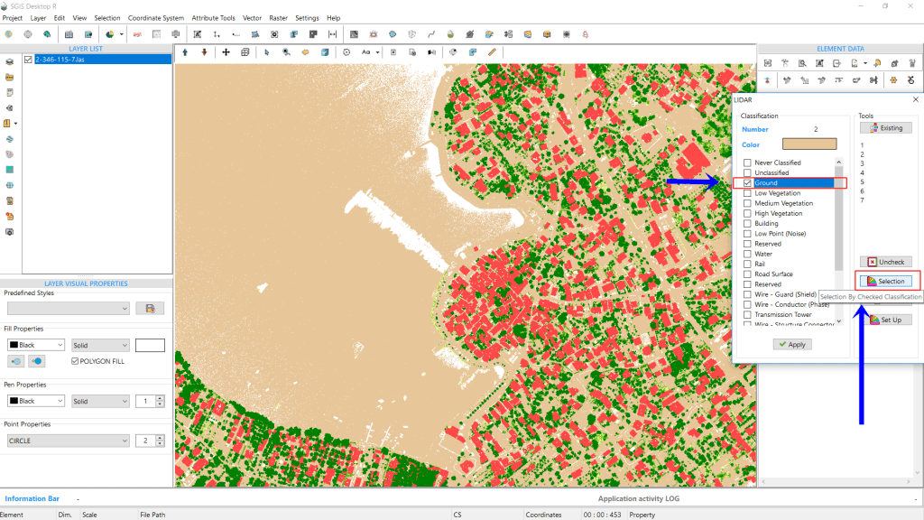
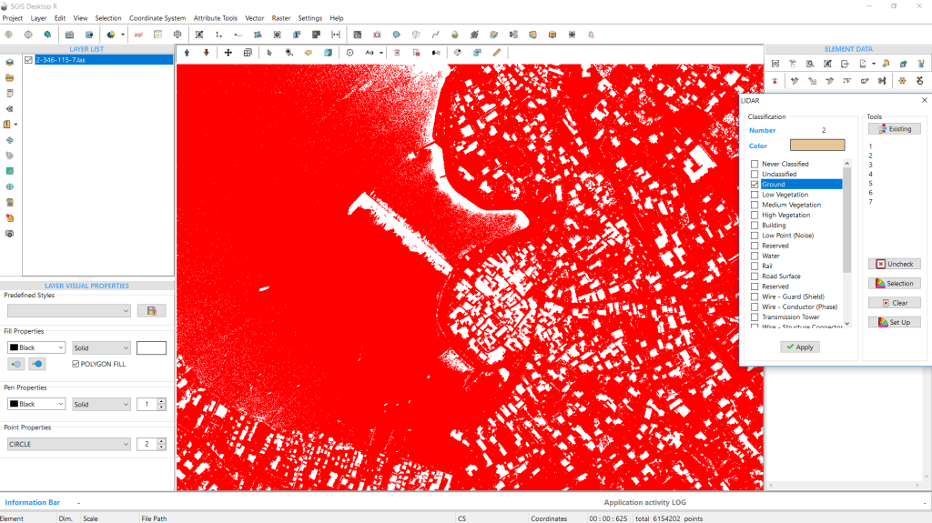
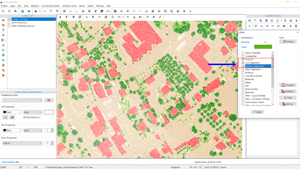
Next, we’ll use the same point cloud to generate a DTM hillshade. Since the LAS point cloud is already imported, we’ll go back to the ‘LIDAR’ toolbox. Here, we’ll ensure that only the ‘Ground’ classification is checked.
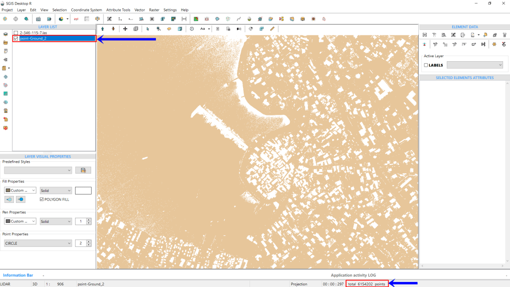
Using the ‘Selection By Checked Classification’ function, we’ll isolate the ground points and create a new GIS layer in the Layers Panel. After clicking ‘Selection,’ we’ll assign a name to the new layer, and it will be generated.
Fig.11 Only the 'Ground' classification is selected to generate the DTM hillshade.
Fig.12 After clicking 'Selection by Checked Classification,' all ground points are selected and highlighted in red within the main graphic window.
The information toolbar in the corner will display the number of points in this ground layer.
Once that’s set, we’ll open the ‘Create Grid’ tool to adjust the settings.
Fig.13 The new Ground layer is created, and the number of points it contains is instantly displayed in the information toolbar at the bottom of the user interface.
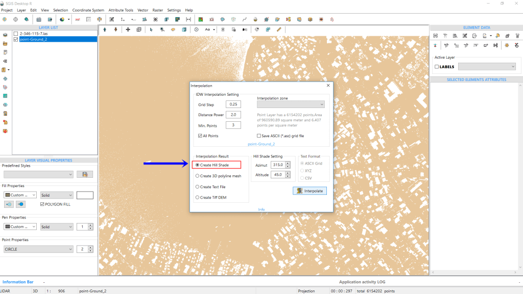
Fig.14 Adjusting the input and output settings in the Interpolation dialog for generating a DTM hillshade: Grid Step set to 0.25m, Distance Power at 2, and Min. Points at 3.
In the Interpolation dialog, we’ll adjust both the input and output settings. Since we’re generating a DTM hillshade, we’ll use the same settings as before. The Grid Step will be set to 0.25m, with the Distance Power at 2 and Min. Points at 3.
For the output, we’ll select ‘Create Hillshade,’ keeping the default Azimuth at 315 degrees and Altitude at 45 degrees. Once everything is set, we’ll click ‘Interpolate’ to generate the hillshade.
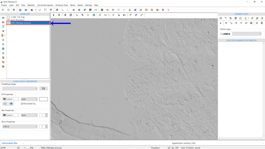
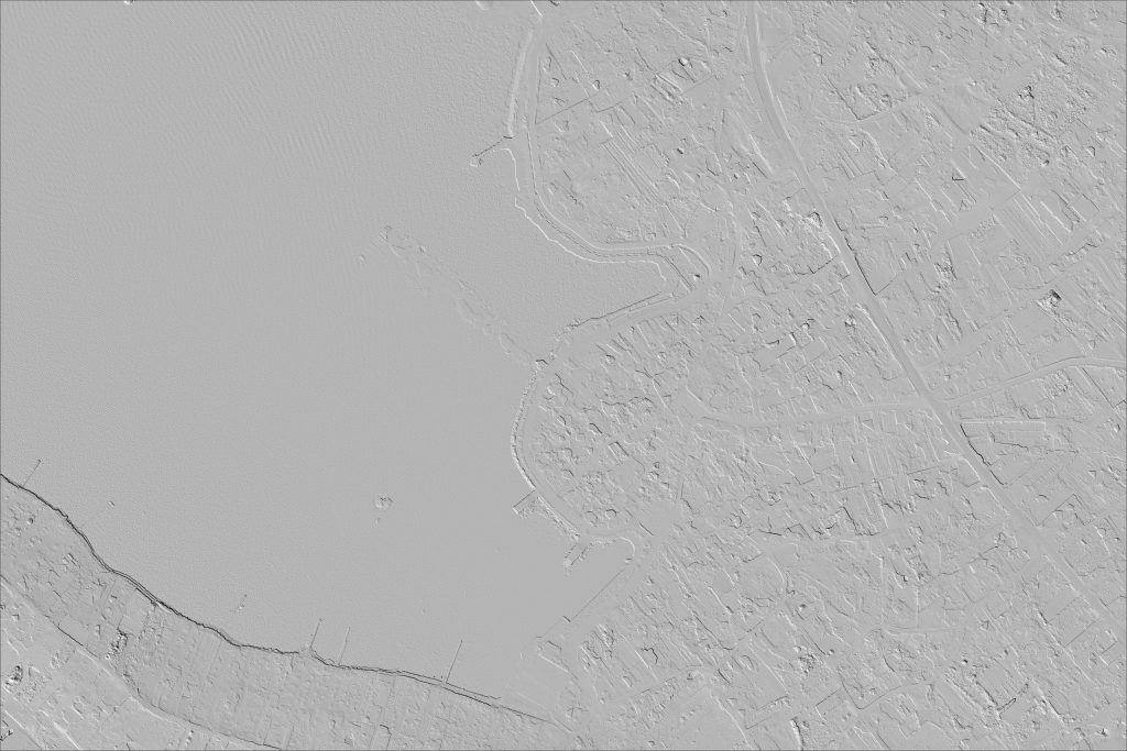
Fig.15 The DTM hillshade has been successfully generated.
Fig.16 Exporting the hillshade as a raster file.
The hillshade can be exported as a raster file in several formats, including PNG, TIFF, JPG, or BMP. Along with the raster file, the software generates a corresponding world file to ensure the hillshade is georeferenced and properly aligned.
Fig.17 The DTM hillshade is exported as a PNG file along with the corresponding .pgw file.
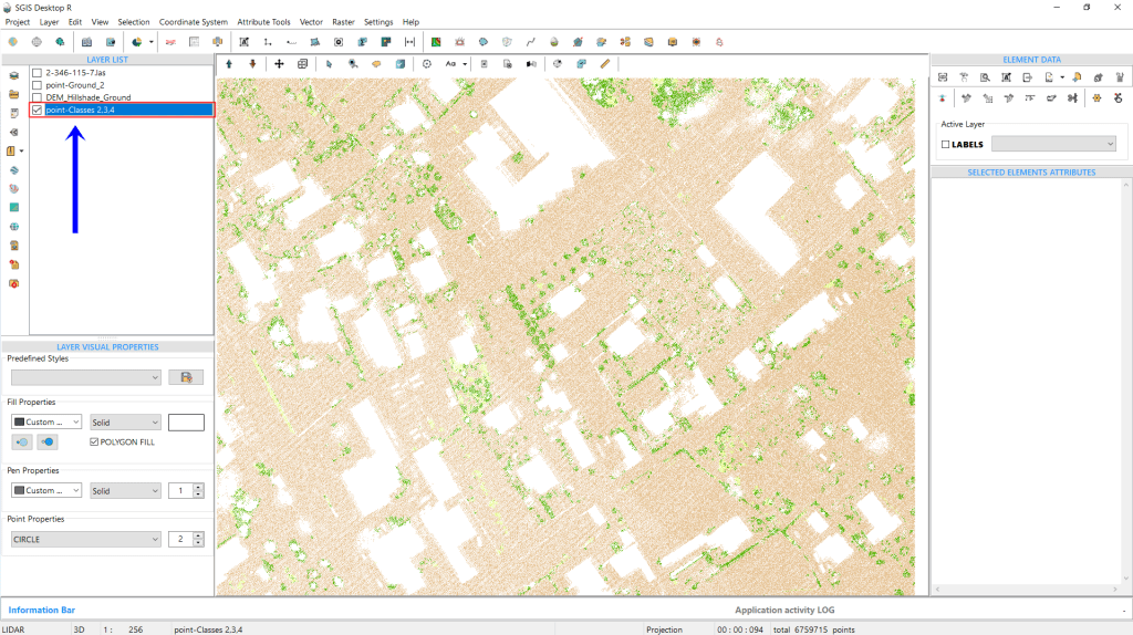
For demonstration purposes, we’ll export a DEM hillshade that includes multiple classifications, such as ground, low, and medium vegetation. This shows that the algorithm can handle combinations of different classifications, not just a single one. The process remains the same, but this time, we’ll keep three classes selected in the ‘LIDAR’ toolbox: 2, 3, and 4.
Fig.18 The algorithm processes multiple classifications (2, 3, and 4) selected in the 'LIDAR' toolbox, demonstrating its ability to handle combined classifications.
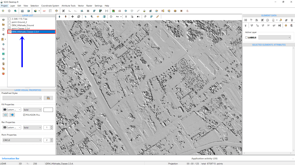
Fig.19 A new layer combining classes 2, 3, and 4 has been created.
Fig.20 A DEM hillshade combining classes 2, 3, and 4 has been generated.
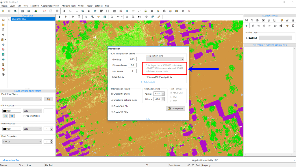
To conclude our analysis, we will add another LAS file, which contains 9,212,883 points covering an area of 249,999.99 m². The average point density is about 36.85 points per square meter, significantly higher than the previous LAS file, where the average was 10.5 points per square meter. With this denser dataset, we can interpolate using a Grid Step of either 0.1m or 0.25m. To determine which provides better results, we’ve exported hillshades for both grid steps.
The results are as follows:
Fig.21 The newly added LAS file contains 9,212,883 points, with an average point density of 36.85 points per square meter over an area of 249,999.99 m².
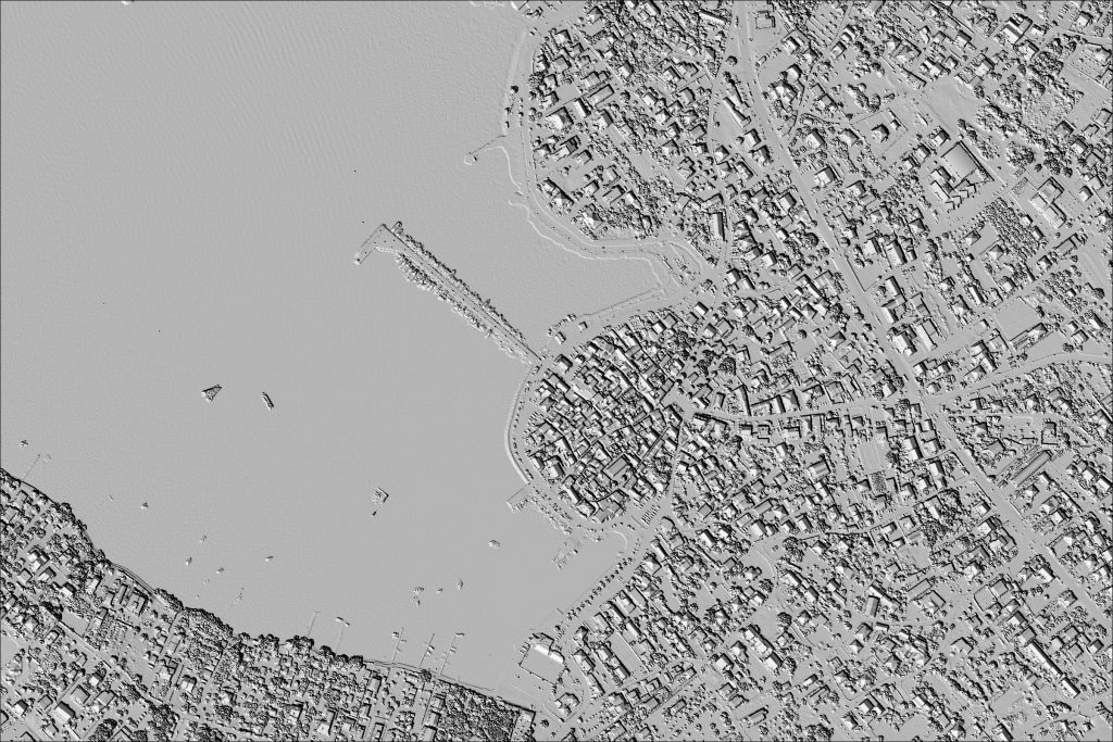
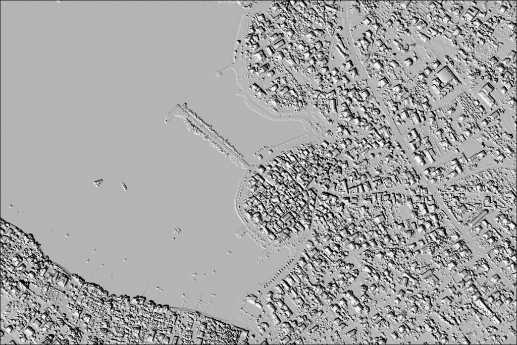
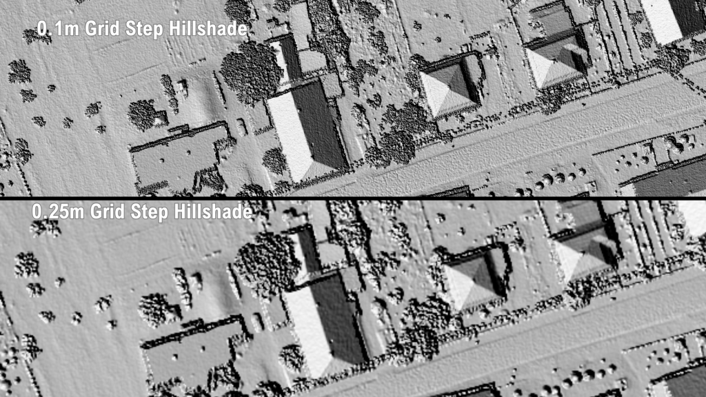
Fig.22 Comparison of hillshades generated with 0.1m and 0.25m grid steps, demonstrating how the 0.1m grid step provides better results for a point density of approximately 37 points per square meter.
With an average point density of around 37 points per square meter, it’s clear that a 0.1m grid step delivers better results. This analysis highlights that a 0.25m grid step isn’t always optimal. The dataset itself determines the ideal grid step for the best output. For a dataset with an average point density of 10.5 points per square meter, the 0.25m grid step offers the best results. Similarly, when working with a denser point cloud—about 37 points per square meter—a 0.1m grid step yields the highest quality hillshade.
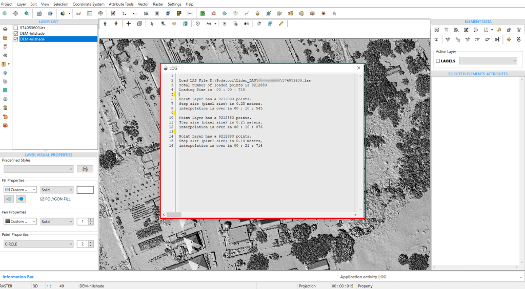
Fig.23 Time comparison from the LOG file, showing that the 0.25m grid step took 10.545 seconds to process, while the 0.1m grid step took 21.714 seconds.
Additionally, the time taken for these processes is noteworthy. From the LOG file, we see that generating a hillshade with a 0.25m grid step took 10 seconds and 545 milliseconds, while the 0.1m grid step took 21 seconds and 714 milliseconds.
To further demonstrate the algorithm’s efficiency across various datasets, we’ll run the procedure using point data collected through GPS-based land survey measurements.