In many GIS systems, polygons must have their exterior rings drawn in a specific direction (typically clockwise) and interior rings (holes) in the opposite direction (typically counterclockwise). Incorrect vertex ordering can lead to polygons rendering incorrectly, appearing inside-out, or causing errors in area calculations. For line features like roads, pipelines, or streams, vertex order dictates the line’s direction, which is crucial for accurate network analysis, flow direction modeling, and other spatial analyses.
Properly ordering vertices ensures topological consistency, maintaining accurate relationships between features such as shared boundaries or connected networks. It also prevents errors that can arise during spatial analysis or when exporting data, ensuring the data remains reliable and usable. In network tracing and flow analysis, the correct vertex order is essential for accurate results. Similarly, GIS operations like buffering or creating offsets rely on the correct orientation of features, and reordering vertices helps achieve the expected outcomes.
Additionally, many GIS projects follow specific standards for how geometries should be stored and displayed. Reordering vertices ensures that your data adheres to these standards, facilitating smooth data exchange and interoperability.
To demonstrate how easy and effective this function is in SGIS v.R, we’ll use a real-world example.
By following these steps in SGIS v.R, you can efficiently reorder vertices and maintain the accuracy and consistency of your spatial data:
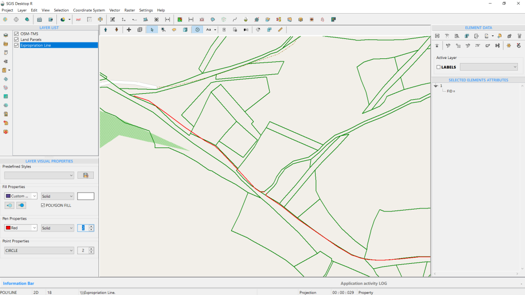
Our example features GIS data with polygons representing land parcels and two separate polylines that need to be connected. To achieve this, we must add an additional vertex and snap it to the starting vertex of the second line.
While this is a straightforward task, the challenge arises because both lines begin at the same point but extend in opposite directions. This scenario highlights the need for a tool that can easily and effectively address such issues.
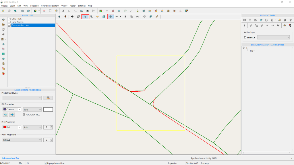
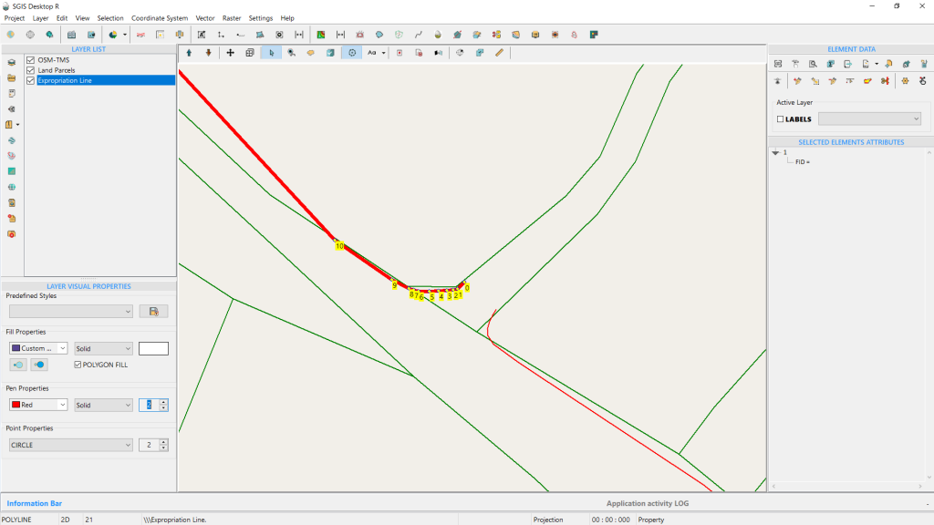
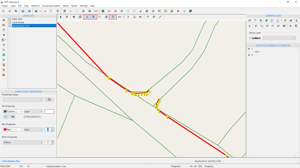
Using the ‘Add to Selection’ Tool, we’ve selected both polylines and displayed their vertices. This highlights the drawing order of each polyline and reveals the gap that needs fixing. Notably, the first polyline is drawn in a clockwise (CW) order, while the second, lower polyline is in a counterclockwise (CCW) order. We need to adjust the vertex orientation of the first polyline to match the CCW direction of the second one.
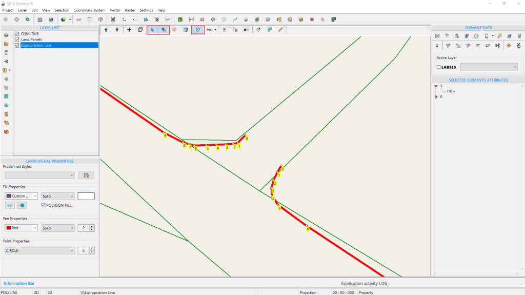
From the Element Data, we access the editing toolbox and select the ‘Add Vertex’ tool. By holding down the Shift key, we activate the snapping option, which is indicated by a red circle around the desired vertex location. The blue arrow pointer highlights the exact spot where we will place the new vertex using the snapping feature.
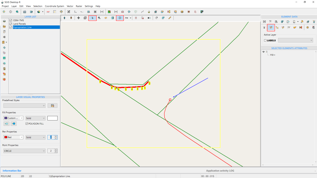
Upon clicking, the new vertex is immediately added. However, since the drawing order is clockwise (CW), the new vertex, numbered 20, connects to vertex 19, which is the last vertex on the upper side.
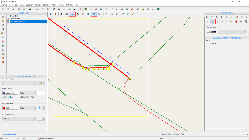
As a result, the line is connected irregularly, visually appearing as if it passes through the polyline feature.
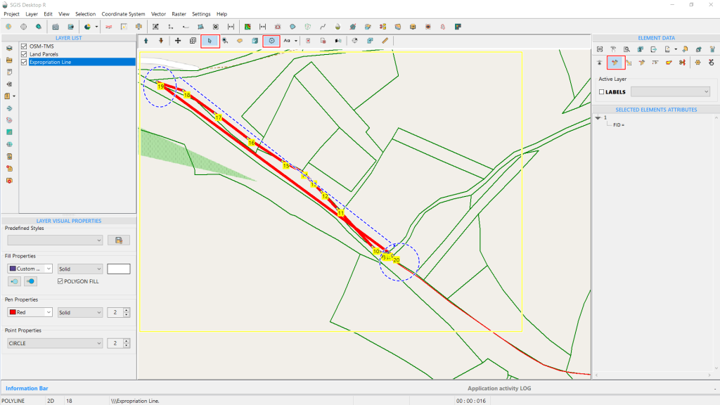
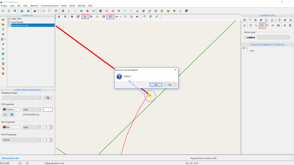
Since this is not the desired outcome, we’ll use the ‘Delete Vertex’ tool from the Editing Toolbox to remove the vertex. The command prompts a confirmation, and we click ‘Yes.’ The procedure is completed, and vertex 20 is deleted.
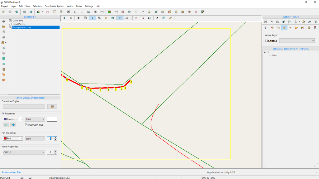
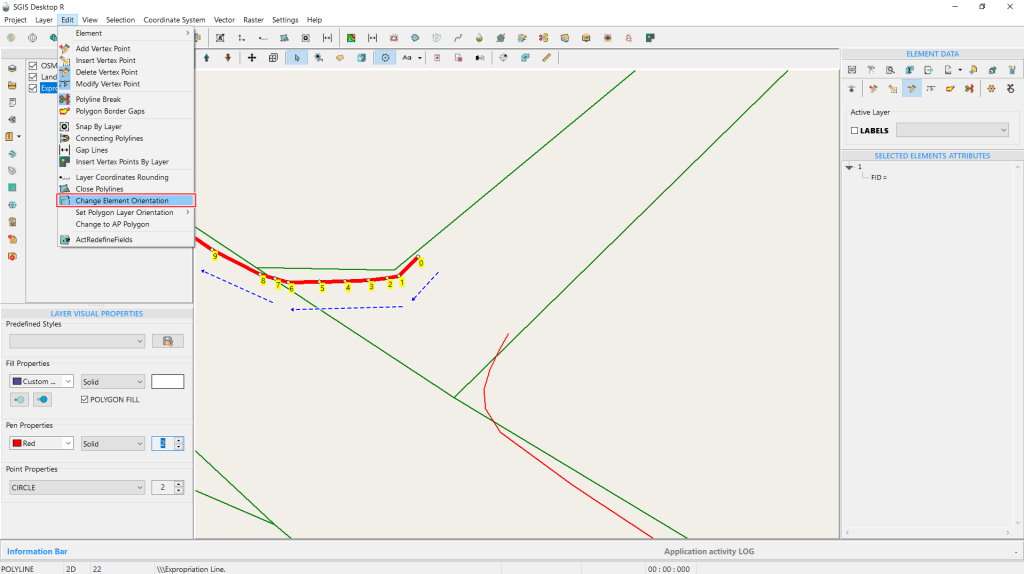
The next step is to open the ‘Change Element Orientation’ function, found in the Edit menu on the Main Menu toolbox. For better visual clarity, it’s highlighted with a red square. On the graphics panel, blue arrows indicate the vertices and their direction before the change.
To begin the process, simply click the ‘Change Element Orientation’ button with the left mouse button.
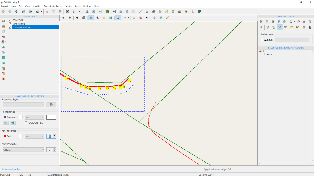
With a single left-click on the function, the procedure is automatically completed. As shown in Fig. 48, the vertices are reordered in the direction indicated by the blue arrows, now in a counterclockwise (CCW) orientation. Note that we need the CCW orientation in this specific example to proceed with the merging process of both lines.
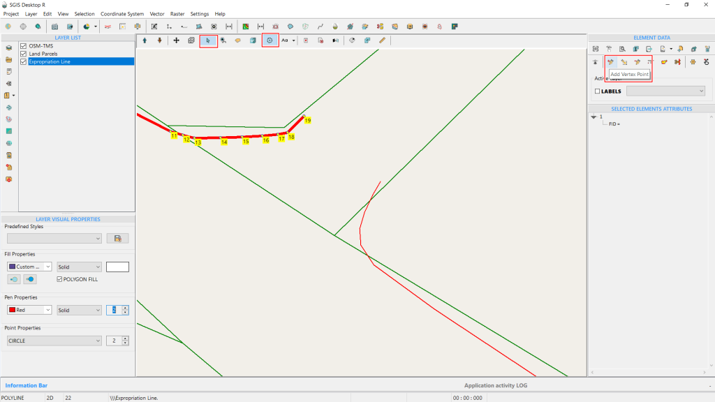
Whether you should use a CW or CCW orientation in GIS depends on the specific application and the rules governing the data, as well as the specific requirements of the GIS project you are working on. There isn’t a universal rule that CW is more accurate; it is about following the correct orientation as per the data standards you are using.
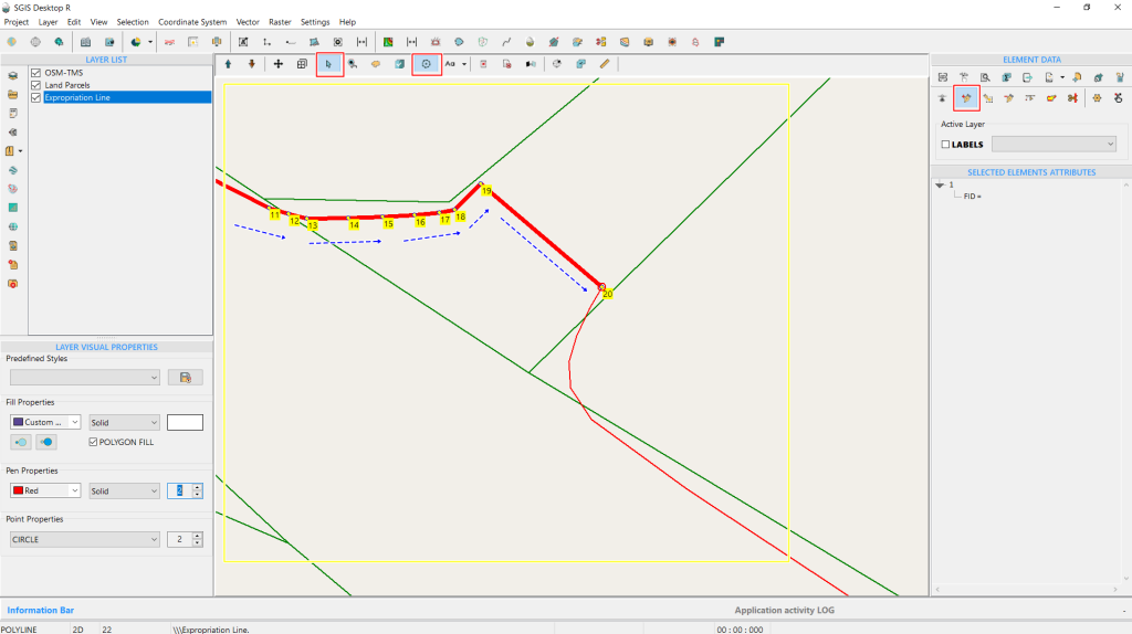
By clicking on the desired vertex and holding the Shift key to activate the snapping option, we place the new vertex accurately. The line is now correctly extended since the vertices are in the proper order. In Fig. 50, this is further highlighted with blue arrows indicating the direction of the polyline.
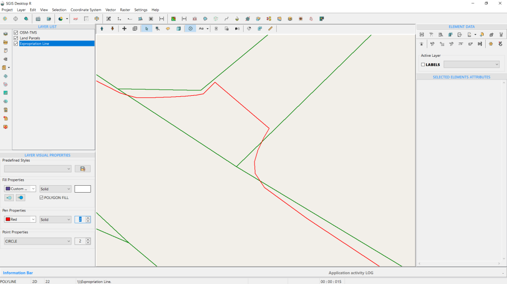
Merging polylines in GIS means consolidating multiple line segments into a single, continuous polyline, reducing complexity and making the data easier to manage and analyze.
In terms of efficiency, this means simplified data editing and processing, as fewer features need to be managed, which can improve the performance of GIS software when handling large datasets.
Merging polylines is generally considered a straightforward task. Most GIS environments offer built-in tools or functions to easily combine multiple line segments into a single polyline. However, the ease of the task can depend on the complexity of the data and the specific requirements, such as ensuring that the lines are correctly aligned or connected before merging.
Let’s start the procedure in SGIS v.R:
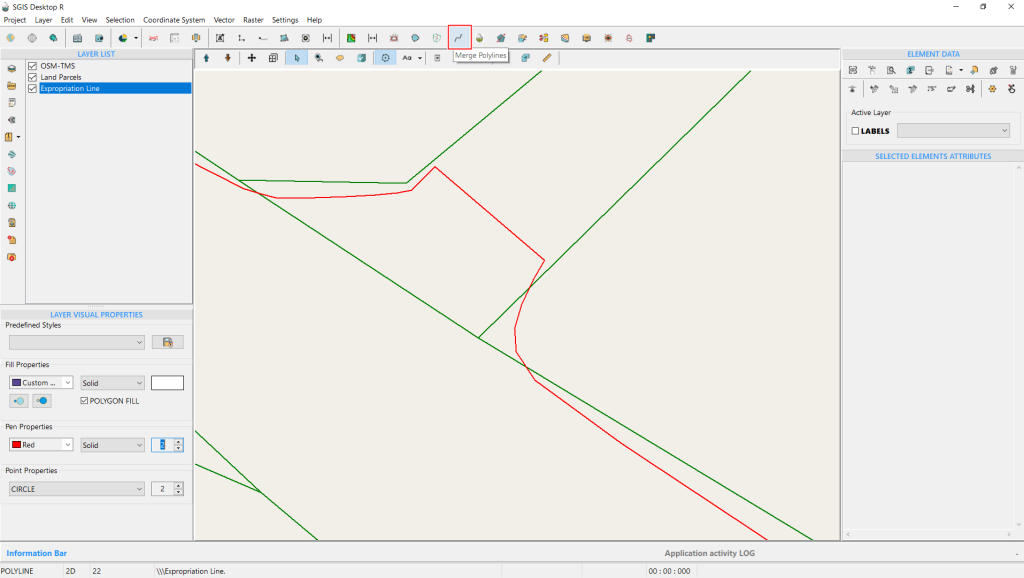
In this example, we’ll continue working with the same dataset from the previous task, where we changed the vertex direction and added an extra vertex to visually close the gap between the two polylines. Now, the logical next step is to merge these polylines into a single, continuous polyline. This is essential because we need one complete polyline feature to later create a buffer polygon from it.
To begin, we’ll access the ‘Merge Polylines’ tool, conveniently located on the main tools ribbon. Click on it to activate the function.
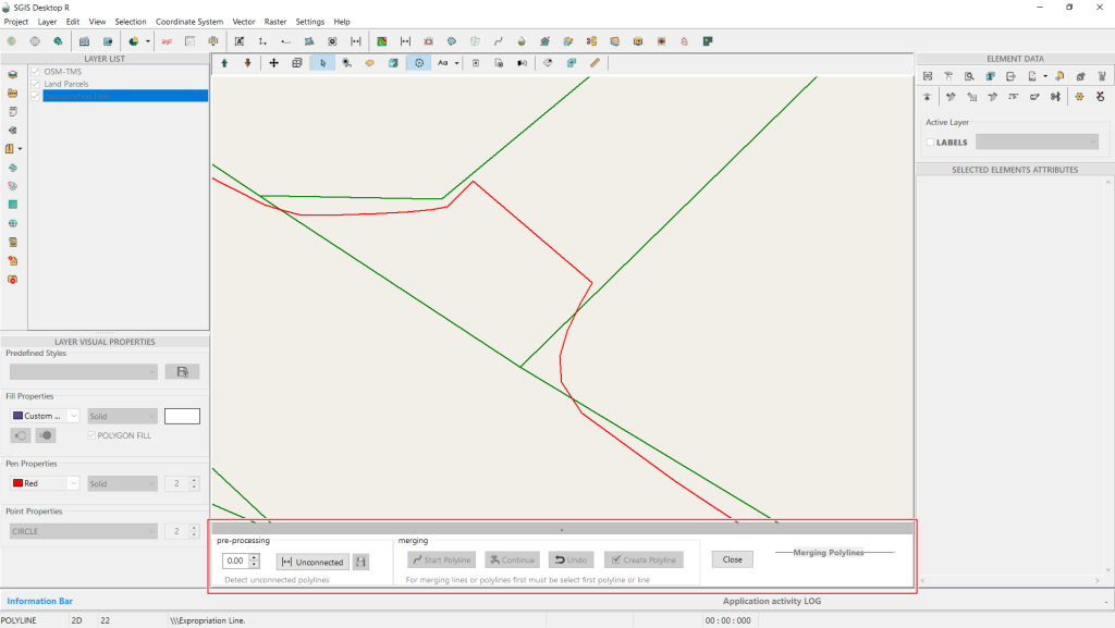
After clicking on the ‘Merge Polyline’ function, a dialog box will appear at the bottom center of the Graphics Panel. This dialog box is essential because SGIS has made the merging process interactive. On the right side of the dialog box, there’s a pre-processing checkup area. Here, you’ll find a numerical input field, which is set to 0.00 by default, and a button labeled ‘Unconnected.’
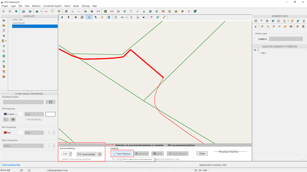
In this step, you can specify the distance within which the software will search for unconnected polylines before starting the merge. After completing the checkup, the function will notify you if there are any unconnected polylines, allowing you to address them before proceeding with the merge.
Since there are no unconnected polylines in our example, we can move on to the next step. First, activate the ‘Select’ function and select the initial polyline feature. Once the first polyline is selected, click on ‘Start Polyline’ to begin the merging process.
Next, select the second polyline and click on ‘Continue.’ The dialog box will prompt you with the message ‘Select and Continue.’
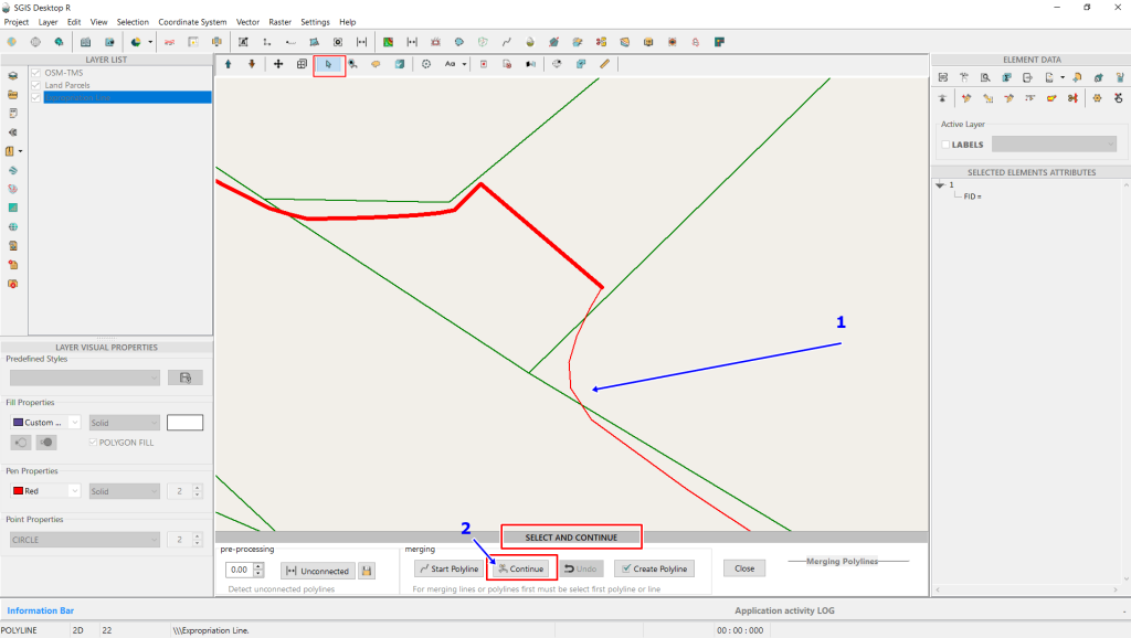
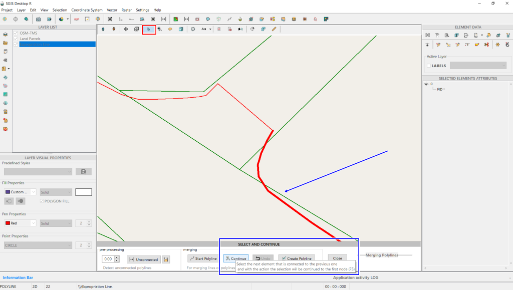
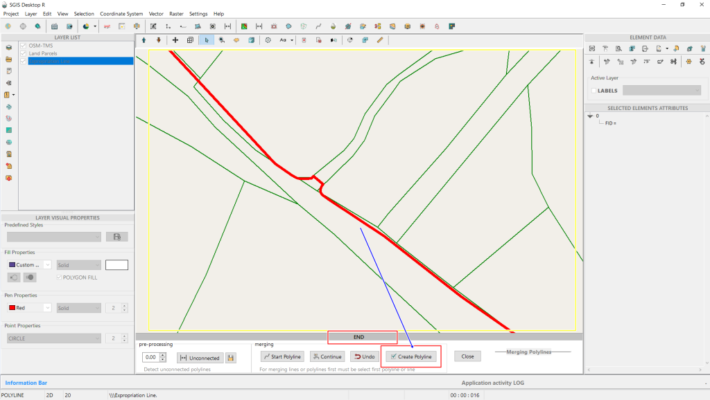
After clicking ‘Continue,’ the entire polyline segment will be automatically highlighted. Since we only have two separate polylines to merge, we click on ‘Create Polyline.’ The dialog ribbon will display ‘END,’ indicating that the algorithm has determined there are no additional polylines to connect.
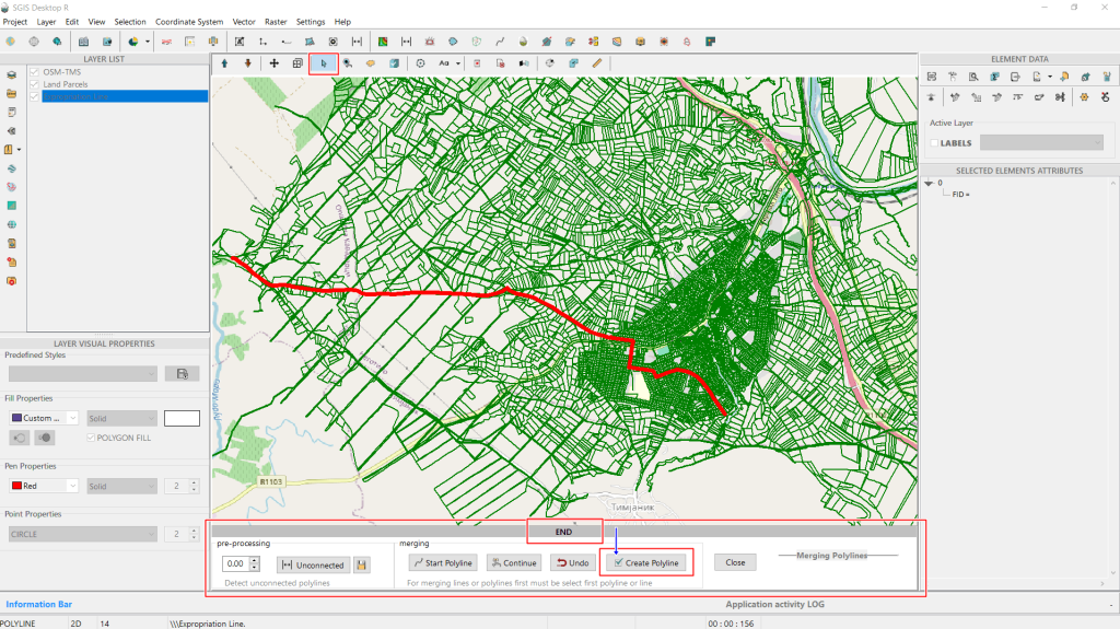
After clicking the ‘Create Polyline’ button, the software will prompt you to name the new layer containing the merged polyline. This ensures that the original polyline layer remains unchanged, while the modifications are saved in a new layer.
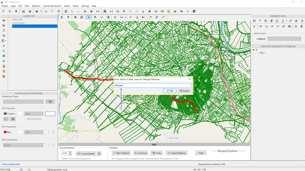
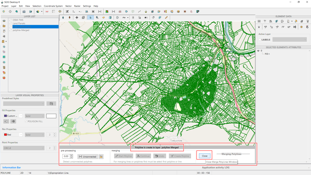
After creating the new layer with the merged polyline, click ‘Close’ to exit the Merging Dialog Box.
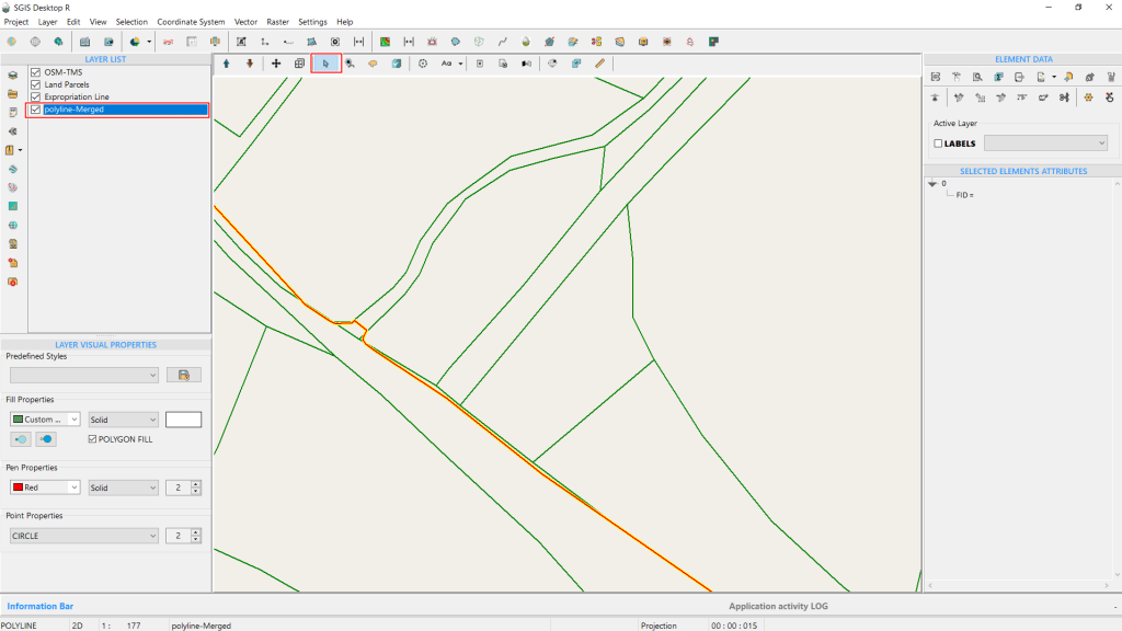
For clarity, we’ll change the original polyline layer to yellow and make it wider, while the newly created merged polyline layer will be colored red. The precise overlap is visible, and selecting the feature will show only one entry in the attribute table.
With this, the procedure is complete.
Buffers help in analyzing areas within a certain distance from a feature, such as finding land within a specified distance from a road or river.
They are used to assess the impact of features on surrounding areas, they allow for spatial queries, enabling users to identify and analyze features that fall within a defined distance from another feature.
In expropriation procedures, buffer polygons are used to determine and manage the areas impacted by the expropriation, ensuring the process is both accurate and fair.
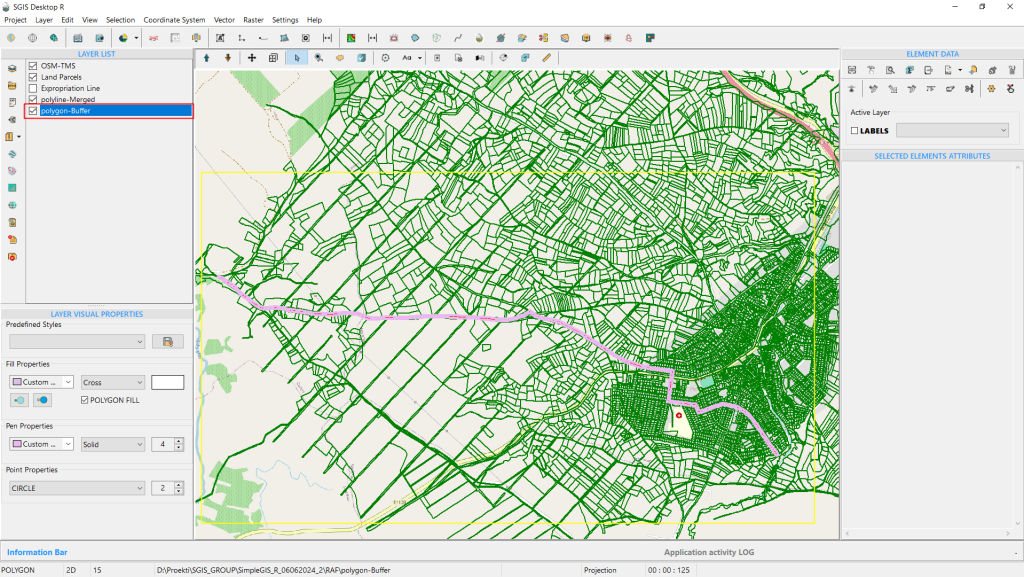
Having made changes to our expropriation line earlier, the next step in this example is to create a buffer polygon. This will help define legal and administrative boundaries for the expropriation process, ensuring that all affected areas are accurately documented and managed according to legal requirements.
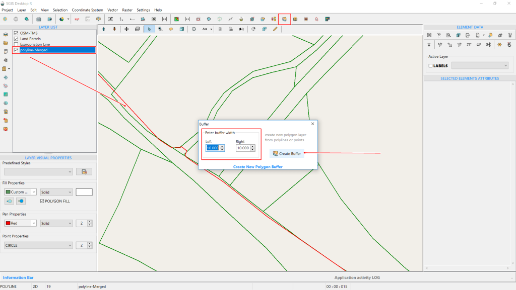
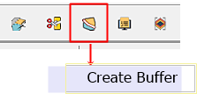
To activate the Buffer dialog window, click on the ‘Create Buffer’ icon on the main tools ribbon. A dialog window will open where you can specify the buffer width. Enter 10 meters for both the left and right sides of the polyline. The description on the right side of the dialog window, ‘Create New Polygon layer from Polylines or Points,’ indicates that buffers can be created from either polyline or point features. Once you’ve set the desired width, click ‘Create Buffer’ to proceed.
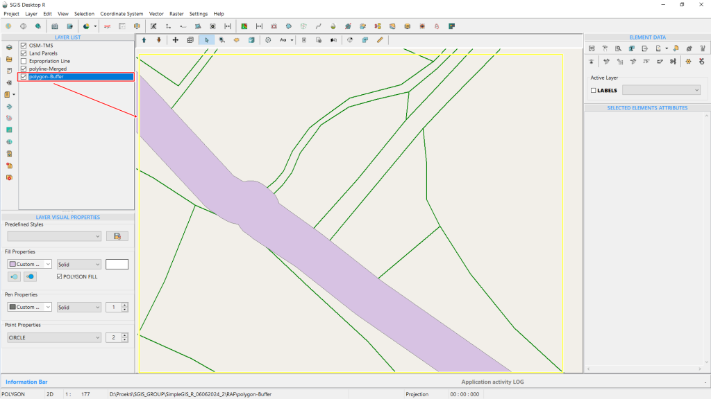
The procedure is now complete, and the buffer polygon is instantly created.
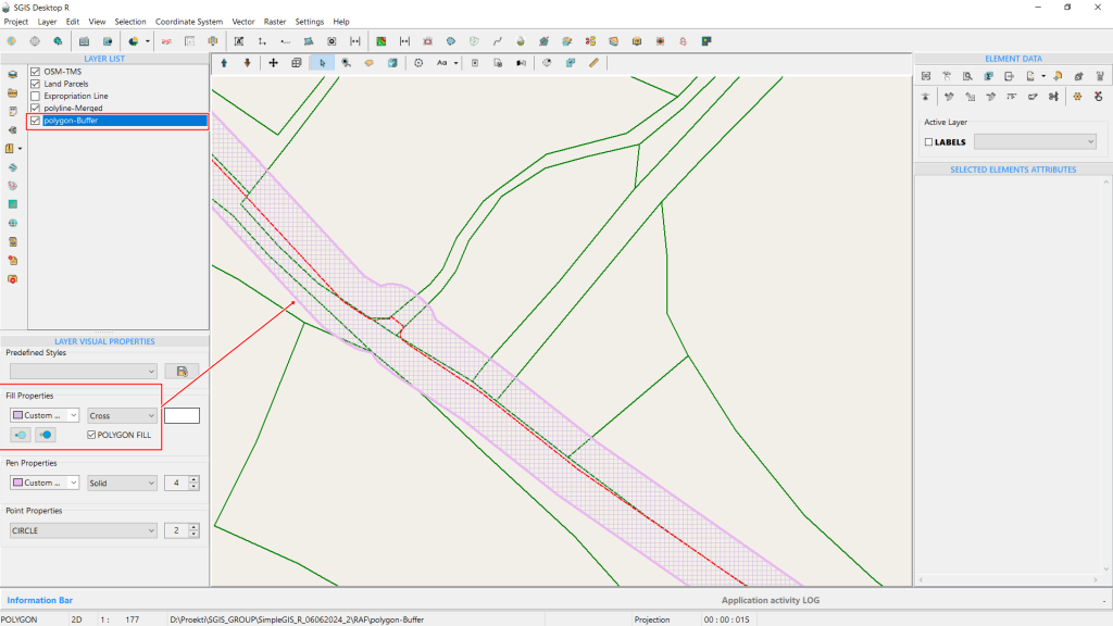
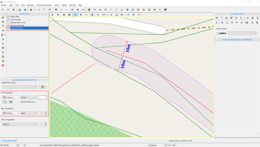
In the ‘Visual Properties’ panel, we change the polygon fill type from solid to cross-hatch, making the polygon transparent. Users can also adjust the colors and other visual styles of the buffer to suit their preferences.
Land Parcel Subdivision is a critical aspect of land surveying and cadastre, involving the legal modification of property boundaries in compliance with local standards and regulations. This process entails dividing a parcel or allotment into smaller lots, each with its own title deed, typically for purposes such as sale, residential development, or ownership transfer.
Given that ownership and parcel characteristics frequently change, it is essential to continuously update the cadaster to align with ongoing subdivision practices.
Land parceling and cadastre updates are not one-time tasks; they are continuous processes because ownership is constantly transferred between legal entities.
Therefore, the ongoing process of subdividing parcels for sale, development, or transfer is crucial and enduring. Each land parcel has legally defined boundaries, documented according to the specific regulations of the country.
In our example involving an expropriation line, we illustrate the importance of land acquisition for infrastructure projects.
Expropriation is the process of resolving property and legal issues related to real estate, such as land and buildings, in connection with the implementation of infrastructure projects.
Infrastructure projects include structures of public interest, such as roads, railways, canals, water supply systems, oil pipelines, sewage systems, gas pipelines, and electrical infrastructure, which may be located either above ground or underground.
To carry out these projects, the boundaries of the designed structure are overlaid onto the cadastral map. This overlap of the existing cadastral state with the projected future state is necessary, to facilitate the sale of land parcels or portions thereof that fall within the boundaries of the planned infrastructure. Such transactions are in the interest of both the project investors and the landowners affected by the construction.
Most infrastructure projects require a continuous piece of land, meaning these projects are typically extensive, crossing multiple parcels and affecting numerous property segments which are often privately owned. Because of this, specialized legal regulations are in place for projects deemed to be of common interest. Without the expropriation process, any landowner could potentially halt the project by refusing to sell or by demanding an unjustifiably high price. Therefore, the expropriation process, and its connection to the land cadastre, is vital for the successful implementation of these projects.
We aim to demonstrate, through a simple example, how SGIS’s algorithm is designed and optimized for fast and efficient performance, particularly given the complexity of the process and the critical importance of the data and outcomes.
This procedure involves dividing the entire project area in one comprehensive process, rather than simply dividing a single parcel into two parts.
In addition, this algorithm not only accurately divides the geometry but is also optimized to recognize and update the attribute table. When a land parcel division is processed in SGIS, the algorithm automatically fills in the attribute table with new area measurements and assigns new numerical labels as Land Parcel Numbers.
In North Macedonia’s official cadastre, the Land Parcel Number is an officially recognized attribute field, included in the data purchased by companies. What makes our algorithm particularly significant is its ability to preserve the historical lineage of cadastral data. When assigning new parcel numbers—such as when a single parcel is divided into two smaller lots—the algorithm does not generate random numbers. Instead, it retains the original number for one lot and assigns a sequential number to the second lot. This approach maintains the continuity and traceability of the land registry system, making it easy to identify the pattern of parcel divisions.
The algorithm is designed to handle this process for any number of parcels simultaneously.
Now, let’s begin with the example.


We have imported a dataset into SGIS v.R that includes Land Parcels and a buffer polygon representing the expropriation area. This buffer intersects multiple parcels, affecting various landowners. To prepare a parcelation report, we need to perform Parcel Division, which will provide a comparison between the current state and a proposed new state. Parcel numbers, which are stored in the attribute field PARCNO (a field created by the official government agency for real estate cadastre), are labeled and made visible on the map.
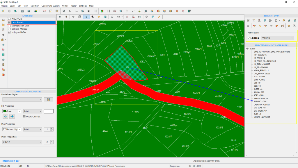

As shown, multiple land parcels are impacted by the expropriation buffer.
When a parcel is selected, its attribute data is displayed, including its area, cadastral municipality, parcel number, land classification, and ownership details.

In this process, we focus on dividing multiple land parcels based on a predefined condition layer, rather than using algorithms that divide by proportional areas or distances. This condition layer is established by professionals for purposes such as the realization of project documentation or urban plans.
The boundaries are carefully checked and drawn based on accurate project documentation.
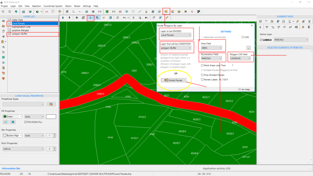
To ensure a smooth process, we first configure the settings in a new dialog box.
Here’s how:
- Select Layer to Divide: Choose the layer you want to divide from the dropdown list. We select the “Land Parcels” layer.
- Set Condition Layer: This determines how the layer will be divided. Our condition layer is the buffer layer, which was created based on the expropriation line and includes a 10-meter buffer on each side, drawn precisely by professionals.
- Define Field for New Areas: Specify the attribute field where the newly created polygon areas will be stored. We use the “Area” field for this purpose.
- Set Numeration Field: This field will store both the original and new parcel numbers for the subdivided lots. It’s crucial for tracking parcel numbers accurately.
- Configure Polygon CM Field: This field helps differentiate polygons, especially in projects spanning multiple cadastral municipalities. We select “CADMUN” (Cadastral Municipality) to ensure unique parcel identification across different municipalities.
Once these settings are configured, click ‘Divide Parcels’ to proceed.

The division process completes in less than a second, as shown in the information ribbon within the ‘Parcel Division’ dialog box. This feature helps users track the time taken for the procedure.
The operation creates a new layer, preserving the original layer intact. All changes are made on the new layer, which appears in the Layers panel as ‘polygon-DP’.
You can adjust its color and visual settings to your preference before continuing.


After completing the procedure, the next step is to export the attribute data for preparing the geodetic report. SGIS simplifies this process by allowing users to export either the entire attribute table or selected features into a CSV file, ready for further processing.
This capability streamlines a task that traditionally required significant time and effort from multiple people, now achievable in just minutes by a single person.

In Fig.77, we see the parcelation of the land parcel numbered 4025/2. The parcel is divided by a red buffer line, with the original number 4025/2 highlighted in white. In the new DP layer, the subdivided parcels are numbered 4025/2 and 4025/3. The original number is retained for the larger portion, while the expropriated section is assigned the new number 4025/3. This method preserves the historical lineage of the parcel, indicating that the newly numbered section was originally part of the larger parcel. This approach is crucial for maintaining the accuracy and continuity of land cadastre and registry systems.
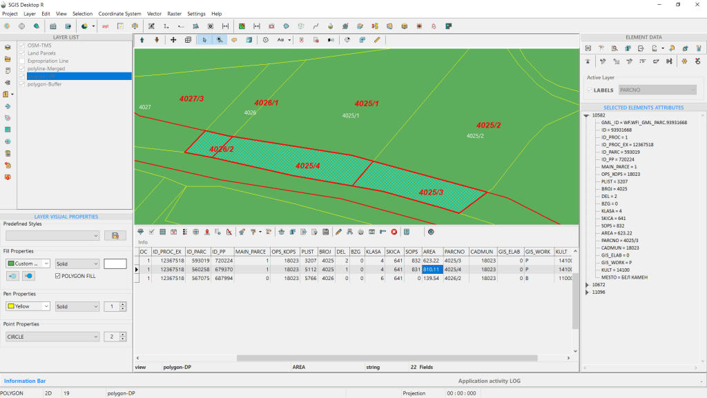
The procedure is now complete.
This method of dividing multiple parcels is designed for processes such as expropriation, urban plan implementation, or any situation where there is an existing cadastral state that needs to be updated to reflect a projected state. Based on the cadastral registry, each landowner will receive appropriate compensation for the acquisition of their land.
Traditionally, this process is done one parcel at a time, but with our algorithm, it is completed simultaneously for all parcels. This approach maintains accuracy, precision, and data integrity while significantly reducing time and resource requirements.
Changing the orientation of a layer from clockwise (CW) to counterclockwise (CCW), or vice versa, is crucial in GIS to ensure that data meets the specific orientation requirements of different software and data standards. Polygon orientation is essential for accurate processing, such as calculating area or performing spatial overlays, and incorrect orientation can lead to topological errors.
For instance, the commonly used shapefile format in GIS typically requires polygon rings to have a clockwise (CW) orientation for exterior boundaries and a counterclockwise (CCW) orientation for interior boundaries (holes). This distinction is important for correctly interpreting and displaying polygons.
In contrast, the GML (Geography Markup Language) format usually requires the opposite orientation: counterclockwise (CCW) for exterior boundaries and clockwise (CW) for interior boundaries, following the “right-hand rule” used in many systems.
Having a tool that can adjust the orientation of an entire layer is therefore extremely useful. It helps ensure that spatial data is consistently interpreted and displayed across different platforms, preventing errors and maintaining data integrity. Let’s dive into our example.
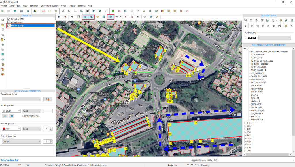
In this example, we’ll start by opening a SHP file that contains two polygon layers: parcels and buildings. Using the ‘Select’ function along with ‘Add to Selection,’ we select several polygons.
It’s important to note that we’re selecting them purely for demonstration purposes, to show how the vertices look before and after the orientation change. The function itself works on the entire layer, so there’s no need to select individual objects or features. The user only needs to ensure the layer is active in the Layers panel, then open and execute the function.
Returning to our example, as seen in Fig. 79, the orientation of the selected polygon vertices is currently clockwise (CW). Our goal is to change the orientation of all features in this layer—specifically, all the buildings—to counterclockwise (CCW).
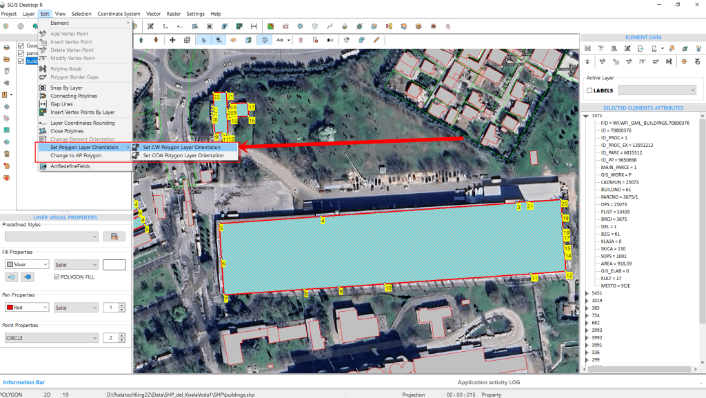
This function provides two options: ‘Set CW Layer Orientation’ and ‘Set CCW Layer Orientation.’ These options standardize the orientation of the entire layer. For instance, if a layer contains polygons with mixed orientations, the function will unify them, making all polygons either CW or CCW, depending on the option selected.
To change the orientation of our SHP layer to CCW, simply click on ‘Set CCW Polygon Layer Orientation,’ and the entire layer will be adjusted accordingly.
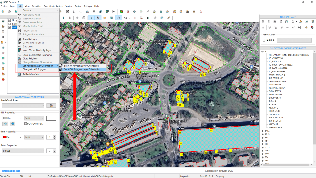
This automatically changes the entire layer to a CCW orientation.
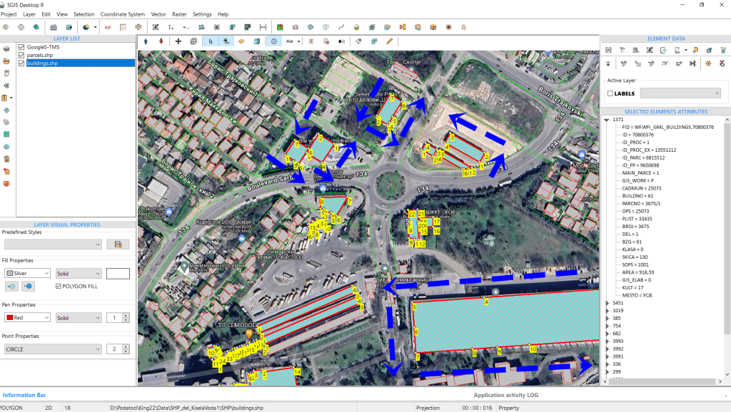
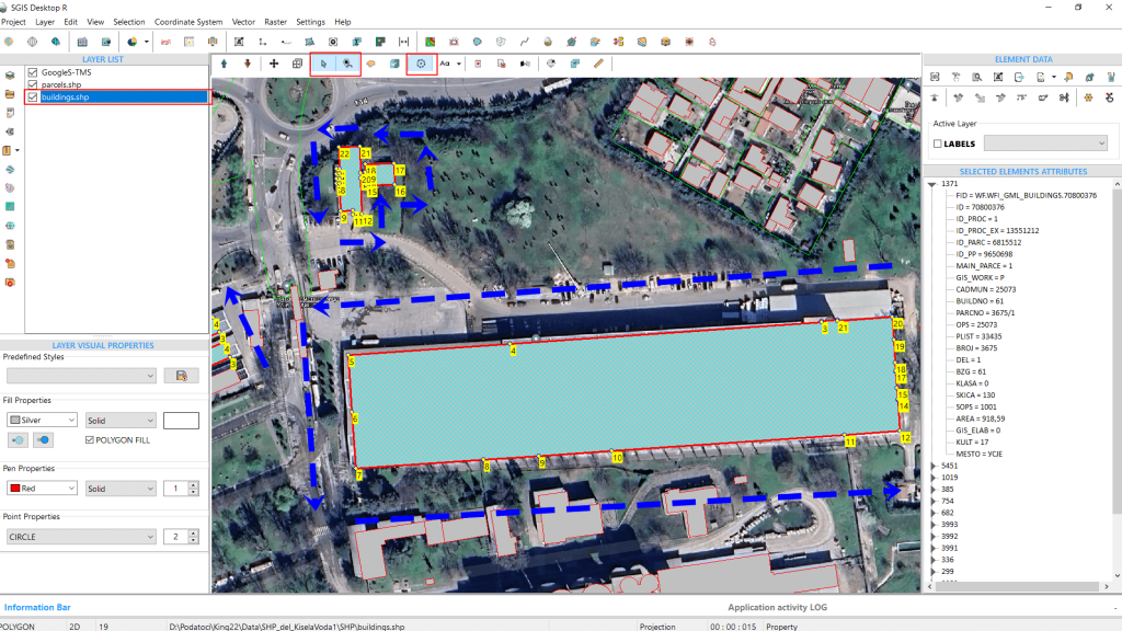
If we need to change the orientation of the entire polygon layer back from CCW to CW, we can easily do so by selecting the ‘Set CW Layer Orientation’ option from the edit menu. With just one click, the layer’s orientation will be adjusted.
In Fig.82, we’ve zoomed in to provide a clearer view of the vertex points for better visualization.
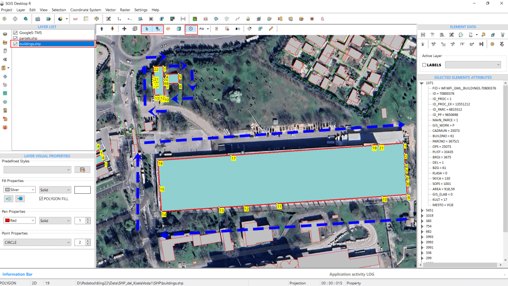
As mentioned earlier, the SHP file format typically requires the outer boundaries of polygons to have a CW orientation, while the GML file format specifies that these boundaries should be in a CCW orientation.
To demonstrate this, we’ll import a GML file from a GML zip archive containing polygons, and then verify and adjust the orientation of the entire layer, switching from CCW to CW and vice versa.
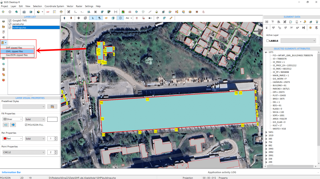
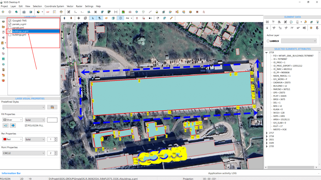
The GML data has been successfully loaded, containing four GML layers of building and parcel polygons. We’ll focus on the ‘buildings_o’ layer. As shown in Fig.86, after loading the data and enabling the ‘Vertex’ function to display vertex numbering, we can immediately see that the layer’s orientation is CCW.
Using the same function, we’ll now switch the orientation to CW.

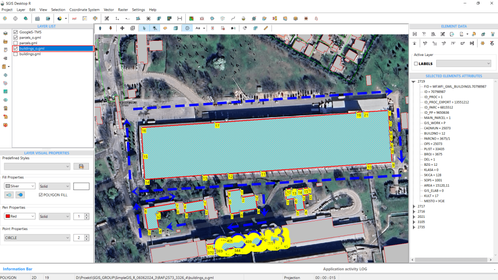
The orientation has been adjusted, and the procedure is complete.
It’s important to note that while this function is available for editing, users aren’t required to use it when saving or exporting their SHP files or other formats. During export, the software automatically saves vertices according to the specifications of the file format.
Rounding decimal values in GIS layers is crucial for standardizing numerical precision across datasets, which ensures consistency in measurements and calculations. This is particularly important when integrating data from various sources. Additionally, certain projects or regulatory standards may require specific levels of precision. For instance, official cadastral records in North Macedonia mandate two decimal places. This function is useful for ensuring that data meets such standards.
We’ll use a real case example to demonstrate how this works in practice.
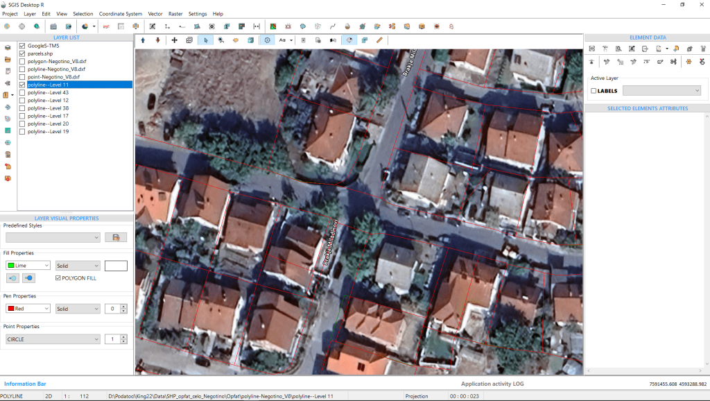
We’ve opened a DXF file containing a parcel layer, along with a Google Satellite base map layer. To compare this drawing with the official cadastral base, we’ll add another layer named ‘Parcels.shp’, which was purchased from the official government portal.
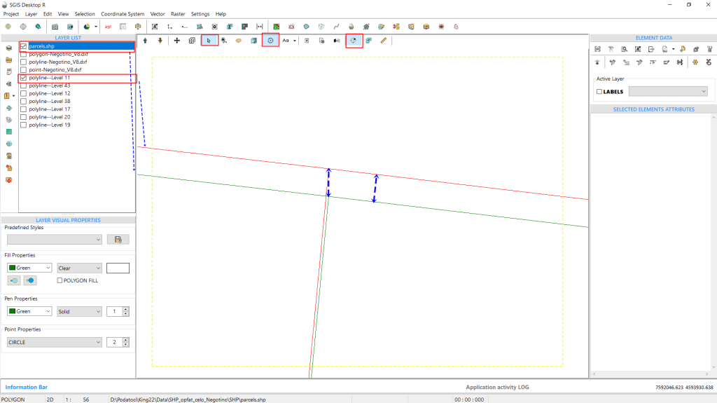
To make the comparison between the vector data clearer, we’ll turn off the base map, allowing us to better observe the layers. At first glance, the layers appear to be identical and overlapping, but a closer zoom reveals that the lines don’t perfectly align.
This discrepancy arises because the official government data requires coordinates to be rounded to two decimal places, while users typically draw with greater precision in GIS or CAD environments. To address this, we’ll round all data in our DXF layer to two decimal places.
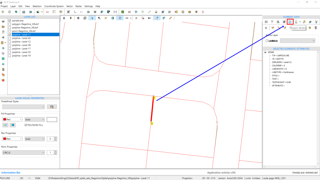
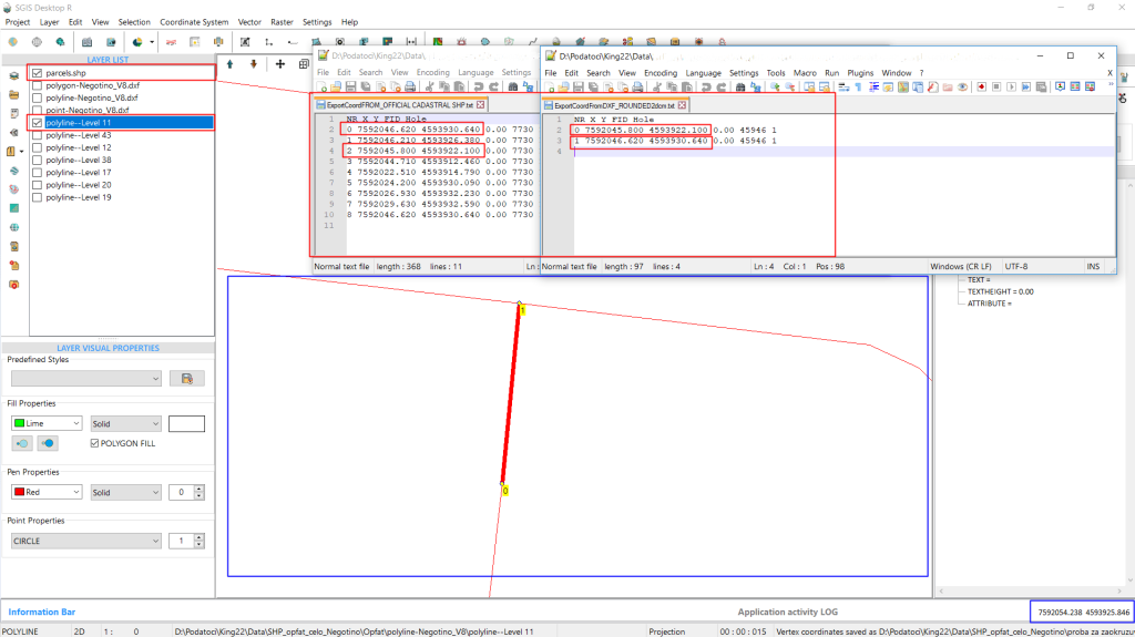
For a before-and-after comparison, we’ll export a set of coordinates from both the user-drawn DXF file and the official cadastral data. We’ll start by selecting a line segment and exporting its two vertices using the ‘Export Vertex’ function. This function opens a dialog box where the user can specify the saving path, separator, and additional export options.
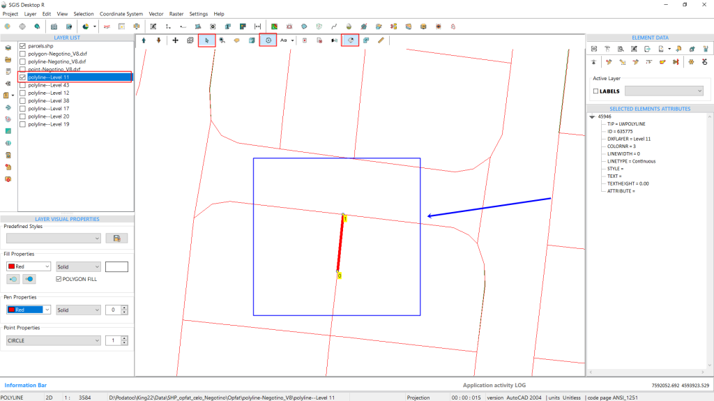
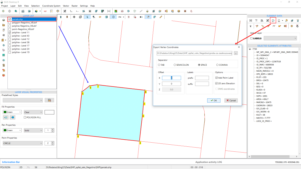
We’ll repeat this process for the cadastral data, which consists of polygons. Although the export will include more vertices, the line from the DXF and the polygon feature should overlap precisely, with two vertices of the polygon coinciding with the two vertices of the line segment we selected.
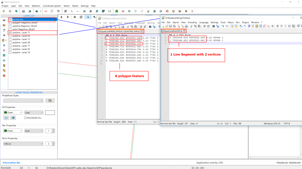
By opening the exported data in a plain text file, we can see that while the difference is small, it is still noticeable. The polygon feature is clearly rounded to two decimal places.
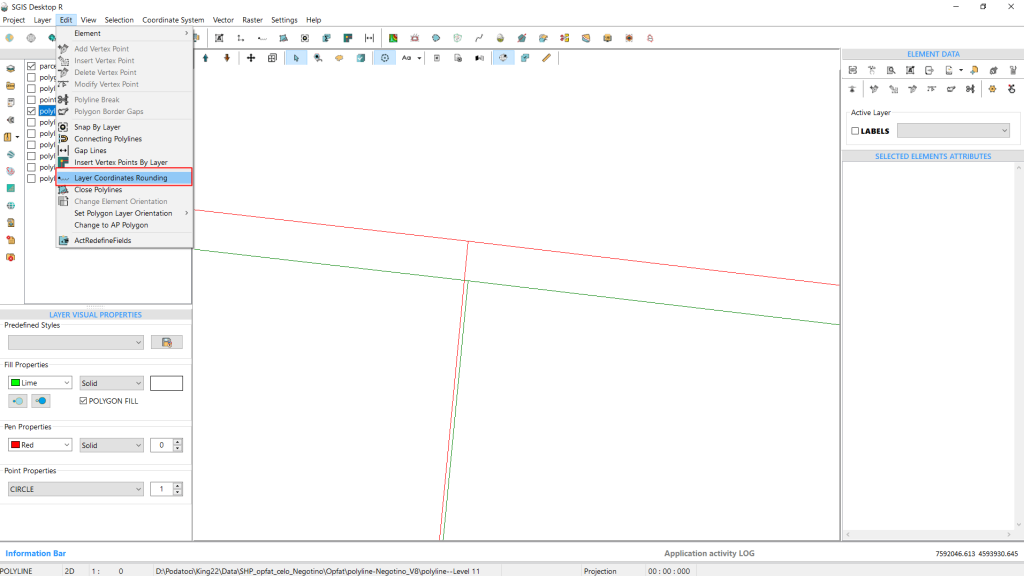
To easily address this, go to the ‘Edit’ menu in the main menu bar and search for ‘Layer Coordinate Rounding’. Click on it with a left click to activate the function.
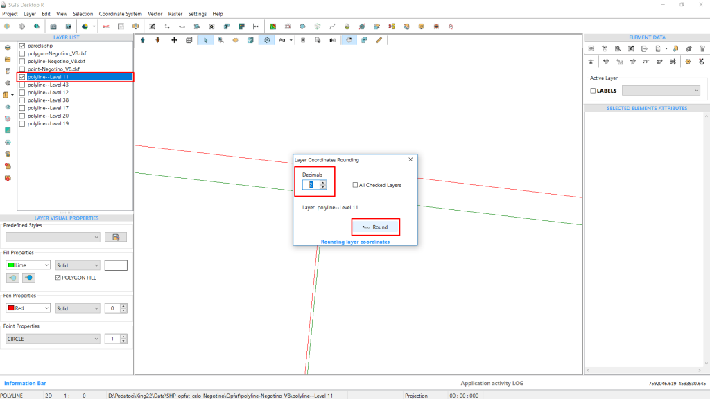
A new dialog window will appear, prompting you to set the number of decimal places needed. In our case, we’ll enter “2.” There’s also an option to check the box labeled ‘All Checked Layers’. If selected, this will apply the rounding to all checked layers in the Layers Panel, adjusting the precision of the coordinates to two decimal places.
If you leave this checkbox unchecked, only the selected layer will be modified, with coordinates rounded to two decimal places. In our example, we’ll leave this box unchecked because we only need to adjust the DXF layer.
Finally, click ‘Round’ to apply the changes.
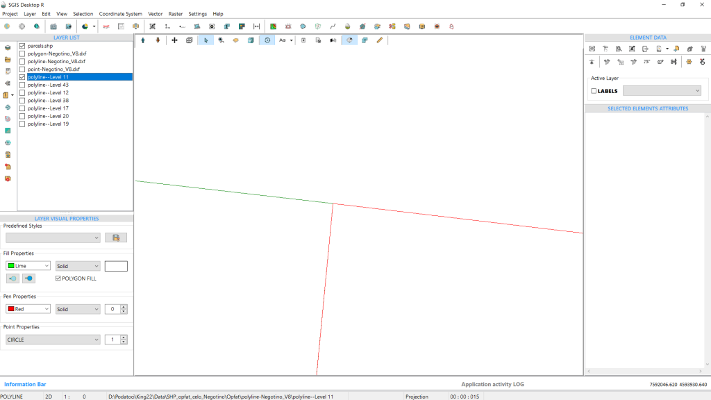
The coordinates match exactly, and this is immediately visible looking at the geometry on the graphics panel. To confirm, we can export the same vertices again and open the files in a text editor. The text editor also shows that the coordinates are identical. With this confirmation, the procedure is complete.
Converting coordinates from Decimal Degrees (DD) to Degrees, Minutes, and Seconds (DMS) format helps align with various systems, standards, and user preferences. Many GIS applications, GPS devices, and mapping software work more effectively with DMS coordinates. Additionally, some mapping or surveying projects require coordinates in DMS format. Therefore, having an easy-to-use tool for this conversion within your GIS environment is very convenient. Let’s explore how this conversion is done in SGIS v.R.
In this example, we have loaded a polygon shape into SGIS v.R that covers an area where we need to extract contour lines. The ‘Real Time Coordinate’ (RTC) function is activated, displaying coordinates in real time as you move the mouse cursor across the graphics panel. These coordinates are shown in the bottom-right corner of the user interface.
To get a better visual preview of the vertices of the shapefile, activate the ‘Vertex’ function. This provides a clear view of the vertex coordinates and their positions.
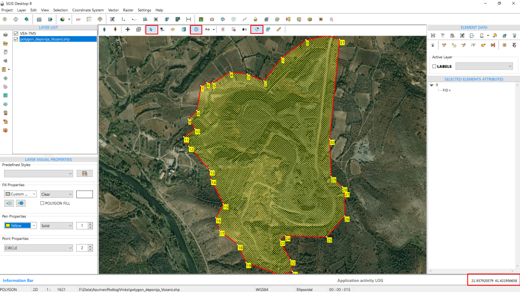
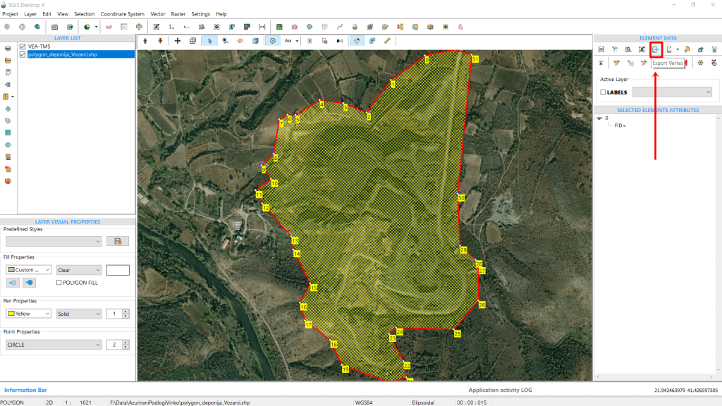
To export these coordinates, which are currently in decimal degrees and WGS84 format, click on the ‘Export Vertex’ function located in the ‘Element Data’ toolbox.
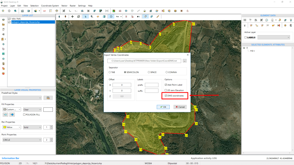
This opens a dialog window where you need to set the separator for the export, which will be saved as a .txt file. In the settings, check the ‘DMS’ coordinate box to convert the coordinates to Degrees, Minutes, and Seconds format. Click ‘OK’ to complete the procedure.
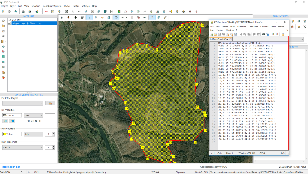
You can verify the results by opening the exported text file in a notepad editor to ensure the coordinates are in the correct format.
This editing task involves adjusting the vertices of features in one layer so that they snap to the points in another layer, using a specific snapping tolerance or condition. By snapping features like lines or polygons to precise points, we ensure that their positions align with more accurate reference data, helping reduce spatial errors. This is especially important when working with datasets from different sources, which often have varying levels of accuracy.
Snapping vertices to a point layer also helps maintain consistency across datasets, which is essential for tasks like overlay analysis, table joins, or building topologically correct models. In networks such as infrastructure, transportation, or utility systems (e.g., roads, pipelines, or cables), snapping ensures that lines connect properly at key points, like intersections or endpoints. This keeps the network intact and enables accurate analysis of connectivity and flow.
For high-precision work—like cadastral mapping or engineering projects—snapping to accurate reference points helps prevent issues with misaligned boundaries or disconnected networks, leading to better decision-making and more reliable results.
To simplify this process, SGIS includes a function that allows users to automatically snap all vertices from one layer to a reference point layer, in addition to manual snapping. This automated cleanup process can significantly reduce the manual effort needed to align large datasets, making data cleaning faster and more productive.

To demonstrate how effective our snapping function is, let’s walk through a real-world example involving an optical cable network polyline layer and a point layer representing field measurements for network maintenance.
In this scenario, we need to verify the positions of the cable network’s vertices, ensuring that they align with the field measurement points. Although there are additional pipelines within the network, they aren’t shown in this example, which is why you’ll see more points than expected.
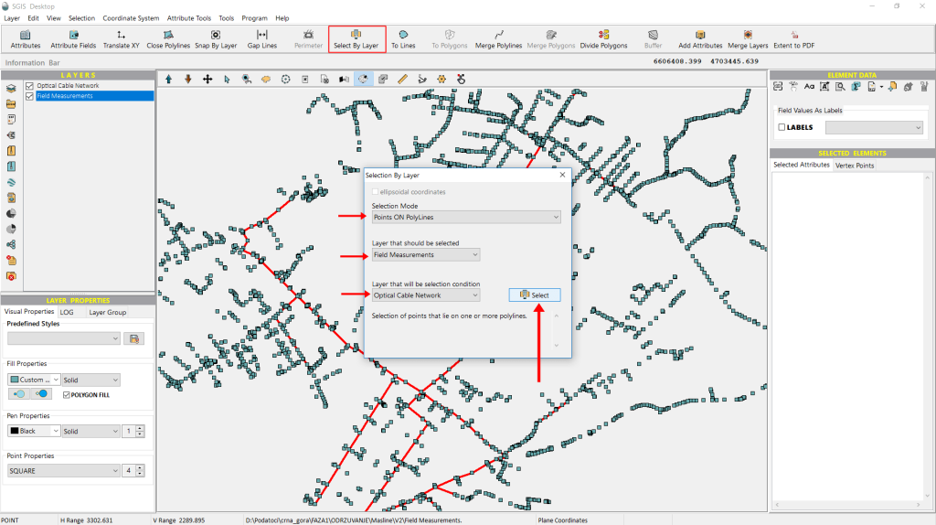
To check if the points and polylines overlap, we’ll use the ‘Select by Layer’ function, which lets us make selections based on a condition layer.
First, we need to choose a ‘Selection Mode’—in this case, we’ll use ‘Points On Polylines’.
Next, we’ll select the layer from which we want to filter point data, which will be the ‘Field Data’.
Finally, we’ll choose the condition layer, which will be the ‘Optical Cable Network’.
Once that’s done, we simply click ‘Select’ to execute the process and check if the points and polylines coincide.
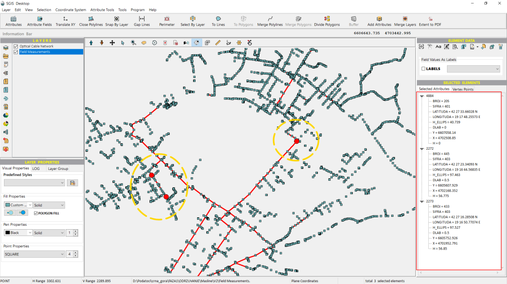
Immediately, the points that meet the specified criteria will be highlighted on the graphics panel.
As shown in Fig. 105, only three points meet our criteria.
Since we require all points to precisely overlap with the polylines, specifically, we need the vertices of the polylines to align exactly with the measurement data points. To achieve this, we will utilize the ‘Snap by Layer’ function.
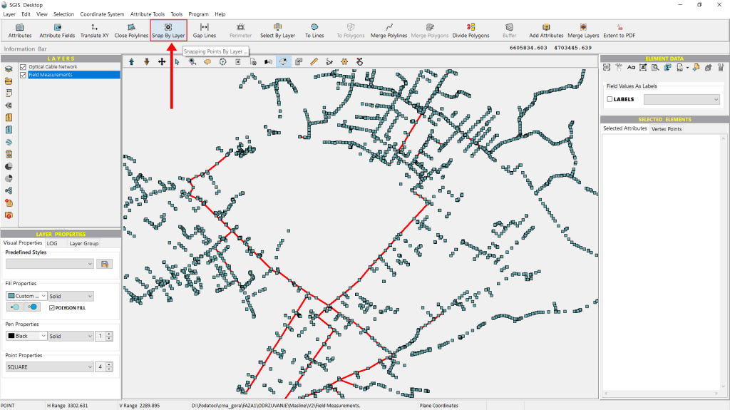
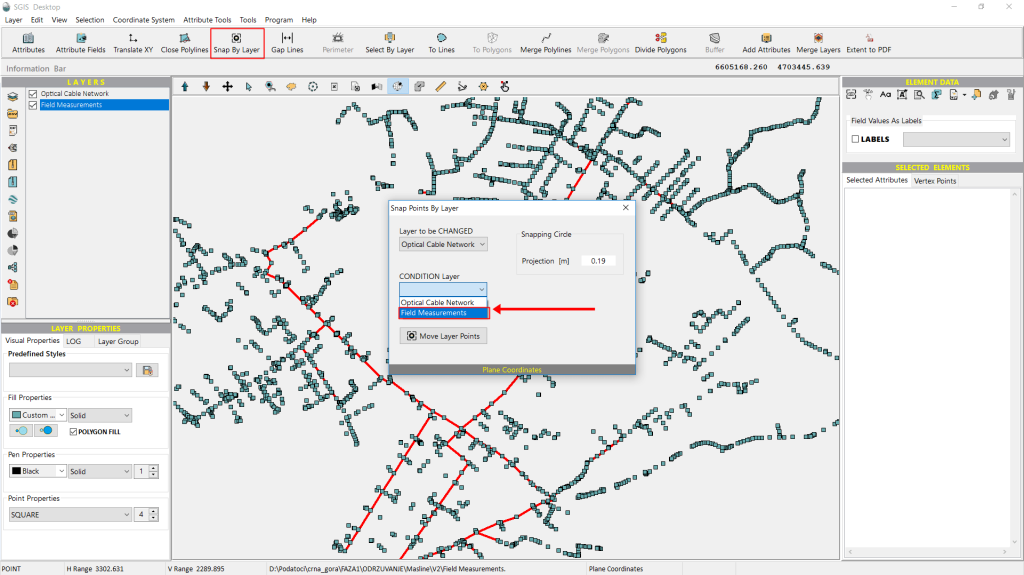
We can find the ‘Snap by Layer’ function on the main toolbar in the user interface. To use it, we just click on the icon.
A new dialog window will appear immediately. In this window, we need to specify which layer we want to modify and which one will serve as the condition layer.
Starting with the first dropdown, for ‘Layer to be changed’, we select ‘Optical Cable Network’.
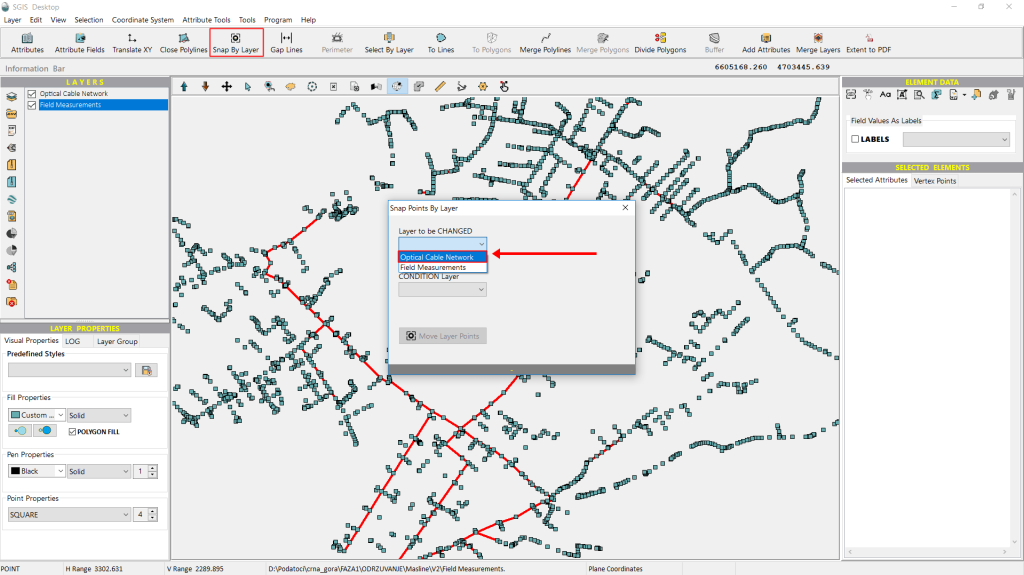
From the ‘Condition Layer’ dropdown list, we select ‘Field Measurements’. This is an easy choice, as there are only two layers loaded in the Layers panel.
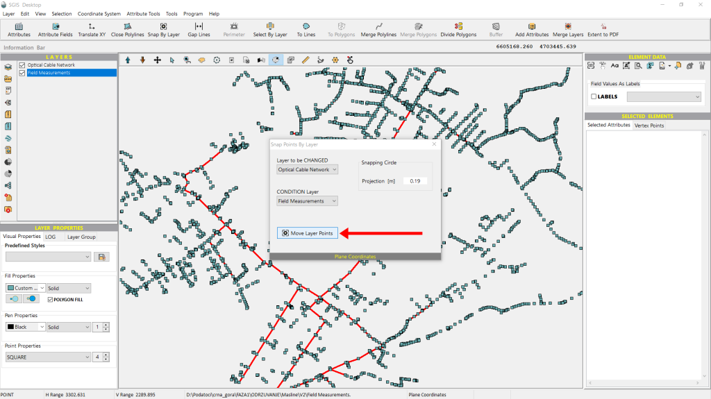
Another setting users can adjust based on their needs is the tolerance gap. This option becomes available after selecting the layer to be modified. Since our layer uses a projected reference system in meters, we’ve set the tolerance gap to 0.19 meters, but this value can be adjusted to suit the user’s requirements.
Once all the settings are configured, we simply click on ‘Move Points’ to apply the changes.
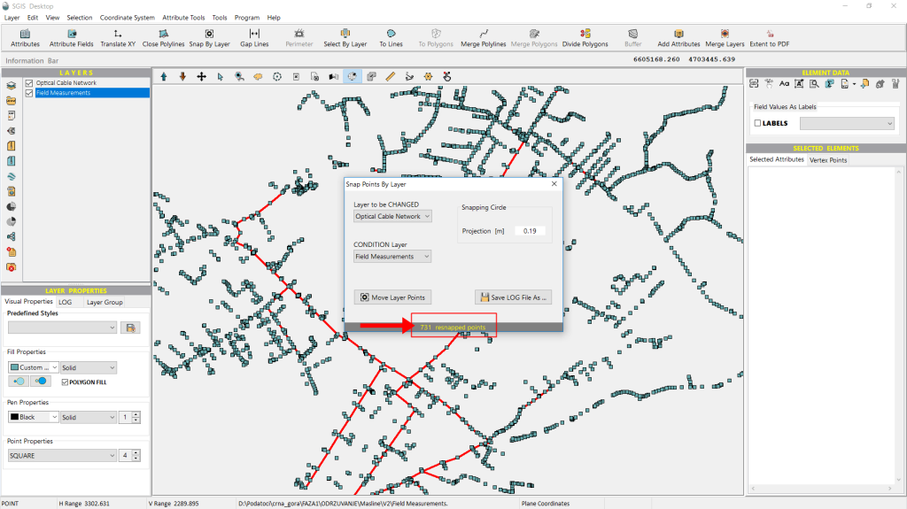
The Info bar at the bottom of the ‘Snap by Layer’ dialog window immediately displays a message indicating how many points have been resnapped.
Now that the procedure is complete and the points have been resnapped in just milliseconds, we can reopen the ‘Select by Layer’ tool to check if the points now align correctly.
We open the ‘Select by Layer’ dialog, configure the settings just as before, and then click ‘Select’ to proceed.
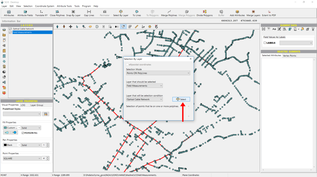
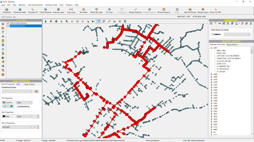
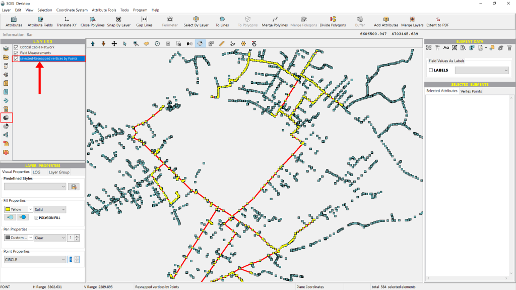
This time, all the points meet the desired criteria and are selected and highlighted in the graphics panel, confirming that they now align perfectly with the field-measured point data after being resnapped.
Additionally, we can export these points to separate them from those that may need modification in the future. This is done using the ‘Selected elements in New Layer’ function, a one-click feature that instantly creates a new layer in the Layers panel. This makes the data ready for export or further processing. With this, the procedure is successfully completed.